Concentration Bounds
Concentration bounds study how likely is that a random variable behaves as expected.
It turns out that, in many relevant cases, random variables concentrate tightly around their expectation. This is particularly true for averages of $n$ idnependent variables, where the bounds concentrate at rate $1 / \sqrt{n}$, and can be used to develop reliable and efficient randomized linear algebra and compression algorithms.
This post focuses on the machinery behind such bounds, covering some popular elements and results from this area, which can then be used to understand and develop tight concentration inequalities. This is structured as a series of sub-sections that are built from first principles and in a linear fashion, culminating with some popular and powerful concentration bounds:
$~$
- Subgaussian/subexponential tails: Mostly definitions. Families of random variables with rapidly decaying probability tails, and some of their main properties
- Moments and moment generating functions: Mostly definitions. These are expectations of variables that give a sense of their “size”, plus some basic properties used later (in particular for sums of independent variables)
- Connecting tail probabilities and expectations: Introducing the basic mechanisms to go from general expectations to probability tails and vice versa
- Connecting tail probabilities and moments: Introducing the basic mechanisms to go from moments to probability tails and vice versa. They form equivalence classes, where slower moment growth corresponds to faster-decaying probability tails.
- Convergence and bounds of MGFs: Unlike moments, the MGF doesn’t always exist. This matters because the existence of a MGF determines whether the Chernoff bound applies efficiently, or inefficiently (2 regimes). This section discusses where the MGF exists, and how do the corresponding bounds relate to probability tail bounds
- MGF-based concentration bounds for sums of independent RVs: We finally discuss bounds for RV sums. The general mechanism is introduced (tail bounds $\to$ MGF bounds $\to$ MGF bound of sum $\to$ Chernoff), and the Hoeffding and Bernstein inequalities are derived as particular instances
The aim is to be a fairly standalone, succinct and easy to follow primer/refresher: derivations, explanations and diagrams favor intuition over rigor. For an exhaustive and rigorous treatment of this topic, a great reference is:
High-Dimensional Probability: An Introduction with Applications in Data Science – Roman Vershynin (Cambridge University Press, 2018 – 2nd ed. 2026)
Subgaussian/Subexponential tails
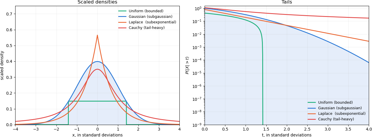
One very useful way to characterize random variables is in terms of their tail bounds, i.e. how quickly does the probability of an event decay as the event goes away from the expectation. Intuitively, if this probability decays faster (i.e. the tail is “thinner”), the random variable is nicer to work with and leads to more “controlled” results. Here, we mostly care about two main categories: subexponential and subgaussian, which can be defined as follows:
Let $X$ be a real-valued random variable obeying the following sub-$\alpha$ tail bound with scale parameter $K$, for all $t \geq 0$: $$ P(|X| \geq t) \leq 2 \exp\Big( - \Big(\frac{t}{K} \Big)^\alpha \Big) $$
The factor of 2 comes from assuming that the bound applies to both tails, i.e. $X$ and $-X$ are sub-$\alpha$ and thus $P(∣X∣ \geq t) \leq 2 \max(P(X \geq t), P(X \leq -t))$. Then, we say that $X$ is:
$~$
- subgaussian if it satisfies the inequality for $\alpha \geq 2$
- subexponential if it satisfies the inequality for $\alpha \geq 1$
Note that these are categories independent of scale: If $X$ obeys the sub-$\alpha$ bound with scale $K$, then any $cX$ also obeys the bound with scale $cK$, and $\alpha$ does not change: $$ P(|cX| \geq t) = P(|X| \geq \tfrac{t}{c}) \leq 2 \exp\Big( - \Big(\frac{t}{cK} \Big)^\alpha \Big) $$
And since $P(|X| \geq t) < P(|cX| \geq t)$ for every $c > 1$, any $K’ \geq K$ satisfies the bound. In fact, the smallest scale that satisfies the bound is equivalent, up to a constant, to the $\alpha$ Orlicz norm of $X$: $$ \lVert X \rVert_{\psi_\alpha} := \inf \Big\{ K > 0 \ : \ \mathbb{E}\Big[ \exp\Big( \Big(\frac{|X|}{K}\Big)^\alpha \Big) \Big] \leq 2 \Big\} $$
This gives us a measure for “to what extent is $X$ sub-$\alpha$”, and will be useful later when adding $n$ independent variables (e.g. establishing that $\alpha$ remains the same, but $K$ grows with $\sqrt{n}$).
Moments and MGF
Moments are particularly useful expectations of a RV, since they are linked to how quickly the probability tails decay: Intuitively, if a distribution has faster decaying tails, the moments will be smaller. Furthermore, the MGF applies nicely to sums of independent RVs: the MGF of the sum is the product of MGFs.
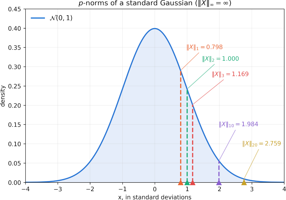
Let $p > 1$ and $X$ be a random variable. Then, the $p$-th absolute moment of $X$ is defined as $\mathbb{E}[|X|^p]$. The $p$-th norm is then $\lVert X \rVert_p = \mathbb{E}[|X|^p]^{\frac{1}{p}}$.
Note that the $1/p$ exponent “brings back” the $p$-th moment to the original scale of $X$: as $p$ grows from 1 to $\infty$, the $p$-norm grows from the absolute mean of $X$ to the maximum value in the domain of $X$. This is known as Lyapunov’s inequality:
$$ \mathbb{E}[|X|] = \lVert X \rVert_1 \leq \lVert X \rVert_2 \leq \dots \lVert X \rVert_\infty = \max(|X|) $$
Let $\lambda \in \mathbb{R}$ and $X$ be a random variable. Then, the MGF of $X$ is: $$ M_X(\lambda) = \mathbb{E}[\exp(\lambda X)] = \sum_{k=0}^\infty \frac{\lambda^k}{k!} \mathbb{E}[X^k] $$ As we can see, the Taylor expansion exposes a weighted sum of all moments, hence the “moment generating” name. The parameter $\lambda$ scales linearly with $X$: $$ M_{cX}(\lambda) = \mathbb{E}[\exp(\lambda cX)] = M_X(c\lambda) $$
But the crucial property we want for concentration bounds is based on the observation that $\mathbb{E}[f(X) g(Y)] = \mathbb{E}[f(X)] \mathbb{E}[g(Y)]$ whenever $X, Y$ are independent. In that case, the MGF of the sum is the product of MGFs: $$ M_{X_1 + X_2 \dots}(\lambda) = \mathbb{E}[\prod_i \exp(\lambda X_i)] \stackrel{!}{=} \prod_i \mathbb{E}(\exp(\lambda X_i)) = \prod_i M_{X_i}(\lambda) $$
Another important property is that, unlike moments, the MGF doesn’t always exist, e.g. the MGF diverges for all sub-$\alpha$ distributions with $\alpha < 1$. This is covered in more detail in the section studying MGF convergence and bounds.
Connecting tail probabilities and expectations
Before studying the MGF, these important and more fundamental building blocks allow us to directly connect the expectation of a nonnegative random variable with its tail probability, a fundamental and useful mechanism.
Let $f_X(x)$ be the probability density function of a nonnegative random variable $X$. Then, the expectation of $X$ can be written in terms of its tail as follows: $$ \begin{align*} \mathbb{E}[X] = &\int_0^\infty x~f(x) dx = \int_0^\infty \Big( \int_0^\infty 1_{t < x} dt \Big) f(x) dx \\ &= \int_0^\infty \Big( \int_0^\infty 1_{t < x} f(x) dx \Big) dt = \int_0^\infty P(x > t) dt \\ \end{align*} $$
Intuitively, it is useful to see $\mathbb{E}$ as a volume integral that can be sliced in two different directions. In one of those directions, slices happen to be tail probabilities (see sketch below).
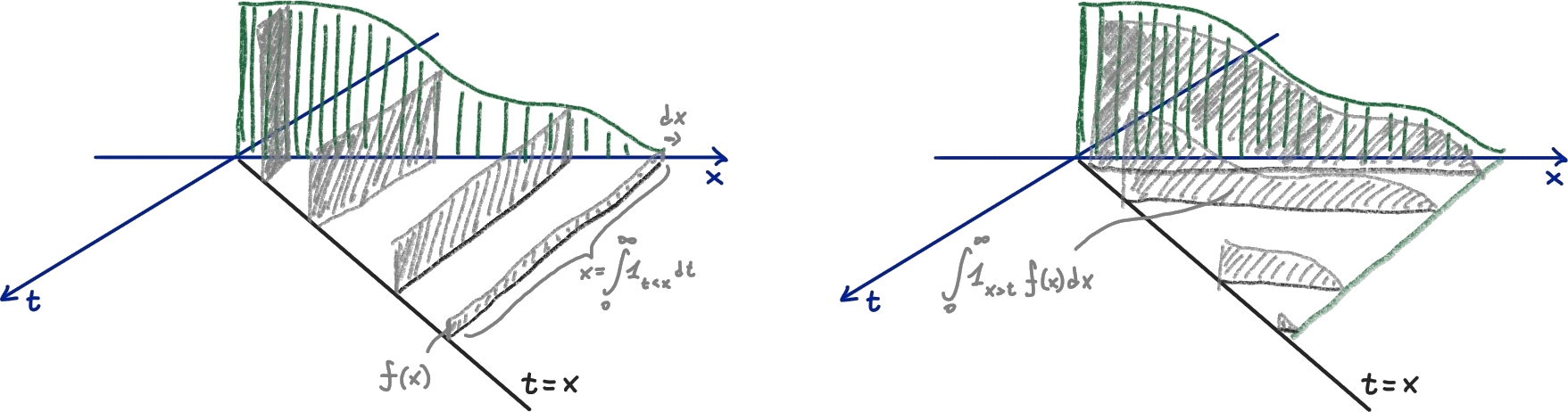
The above layer cake is an equality, another useful and fundamental tool is an inequality:
Let $a > 0$ and $X$ be a nonnegative random variable. Then, $$ P(X \geq a) \leq \frac{\mathbb{E}[X]}{a} $$ Since (given $f(x)$ as the probability density function of $X$): $$ \mathbb{E}[X] \geq \int_a^\infty x f(x) dx \geq \int_a^\infty a f(x) dx = a P(X \geq a) $$
The right-hand side sketch above also helps understanding $\mathbb{E}[X] \geq a P(X\geq a)$. First note that the expectation is the total volume, i.e. we add all “cake layers” for every value of $t$. Now pick $a$ as some fixed value for $t$. It is clear that the corresponding “cake layer”, times $a$, cannot be bigger than the total volume. But it can in fact be equal: If $P(X = 0) = 1 - \mu$ and $P(X = a) = \mu$, we have $\mathbb{E}[X] = \mu a$ and $P(X \geq a) = \mu$, satisfying the equality (this breaks as soon as $X$ has density outside of those 2 points).
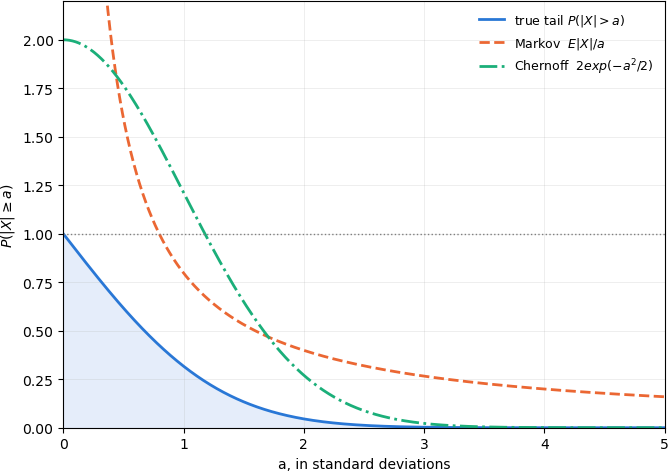
While the Markov tail bound of $\mathcal{O}(1 / a)$ is tight in general, it can still be quite inefficient if we know that $X$ decays faster than $1/a$. For example, if $X$ is standard Gaussian, the probability for a $5\sigma$ tail is approximately 1 in 2 million, but the Markov pobability bound sits at $\sim$20%, way larger. We can make the bound sharper if we inject knowledge about how fast the tails decay. Chernoff’s inequality does precisely this, via the MGF:
Let $a, \lambda > 0$. Then, $$ P(X \geq a) \leq e^{- \lambda a} M_X(\lambda) $$ Where $M_X(\lambda) = \mathbb{E}[e^{\lambda X}]$ is the MGF of $X$. Since we are free to choose $\lambda$, it is typically implied that Chernoff uses the tightest parametrization satisfying $\arg \min_\lambda e^{-\lambda a} M_X(\lambda)$, more commonly in its log-form: $$ \arg \min_\lambda \log(M_X(\lambda)) - \lambda a $$
But let’s first see where does the inequality come from. If we define $Y = e^{\lambda X}$, we have $P(X \geq a) = P(Y \geq e^{\lambda a})$ and $\mathbb{E}[Y] = M_X(\lambda)$. We then apply Markov’s inequality to $Y$ and replace both sides: $$ P(Y \geq e^{\lambda a}) \leq \frac{\mathbb{E}[Y]}{e^{\lambda a}} \Rightarrow P(X \geq a) \leq e^{-\lambda a} M_X(\lambda) $$
Note how we still have a tail bound for $X > a$, but this is now expressed in terms of $M_X(\lambda)$, and it is true for every $\lambda$ as long as $M_X(\lambda)$ exists:
$~$
- If we know $M_X(\lambda)$ is small, this sharpens Markov
- The optimal $\arg \min_\lambda e^{-\lambda a} M_X(\lambda)$ can be often found analytically, such as for subexponential/subgaussian distributions (we’ll do that below)
Let’s visualize this for $|X|$, where $X$ is standard Gaussian and we know the optimal MGF: For this, it can be shown that $M_X(\lambda) = M_{-X}(-\lambda) = e^{\lambda^2 / 2}$, and that it is minimized at $\lambda=a$. The corresponding Chernoff bound reads $P(X \geq a) \leq e^{−a^2/2}$, yielding $P(|X| \geq a) \leq 2 e^{−a^2/2}$ via symmetry of $M_X$ and union bound:
Connecting tail probabilities and moments
Let’s start assuming $X$ obeys a sub-$\alpha$ tail bound with some scale $K$. Can we use this information to find bounds for its $p$-th moment and vice versa? The following block shows that faster decaying tail bounds translate into more slowly increasing moment bounds.
Let $X$ obey $P(|X| \geq s) \leq 2 e^{-(s/K)^\alpha}$. We seek bounds for its $p$-th moment ($p \geq 1$) depending on $K, \alpha$.
We start by applying the layer cake identity to the definition of the $p$-th absolute moment. This exposes the $t^{1/p}$-tail probability of $|X|$, which we reparametrize via $t = s^p$ and $dt = p s^{p-1} ds$: $$ \begin{align*} \mathbb{E}[|X|^p] = \int_0^\infty P(|X|^p \geq t) dt = &\int_0^\infty P(|X| \geq t^{1/p}) dt \\ = & \int_0^\infty P(|X| \geq s) p s^{p-1} ds \end{align*} $$ Now we can apply the assumed tail bound and further reparametrize via $u = (s/K)^\alpha$, i.e. $s = K u^{1/\alpha}$ and $ds = \tfrac{K}{\alpha} u^{\tfrac{1}{\alpha} - 1} du$, which simplifies to the Gamma integral: $$ \begin{align*} \mathbb{E}[|X|^p] \leq & 2 p \int_0^\infty s^{p-1} e^{- (s/K)^\alpha} ds = 2 p \int_0^\infty K^{p-1} u^{\frac{p - 1}{\alpha}} e^{-u} \frac{K}{\alpha} u^{\frac{1}{\alpha} - 1} du \\ = & 2 p \frac{K^p}{\alpha} \underbrace{\int_0^\infty u^{\frac{p}{\alpha} - 1} e^{-u} du}_{\Gamma(\frac{p}{\alpha})} = \frac{2p}{\alpha} K^p \Gamma(\frac{p}{\alpha}) \end{align*} $$ Finally, we apply Stirling’s approximation $\Gamma(z) \approx \sqrt{2\pi / z} (z / e)^z$. We also obtain a bound for the $p$-norm by taking the $p$-th root: $$ \begin{align*} \mathbb{E}[|X|^p] \lesssim &\frac{2p}{\alpha}K^p \sqrt{\frac{2 \pi \alpha}{p}} \Big( \frac{p}{e \alpha}\Big)^{\frac{p}{\alpha}} \\ \lVert X \rVert_p \lesssim & \underbrace{\Big( \frac{2p}{\alpha} \Big)^{\frac{1}{p}} \Big(\frac{2 \pi \alpha}{p} \Big)^{\frac{1}{2p}}}_{\text{goes to 1 as } p \to \infty} K \Big( \frac{p}{e \alpha}\Big)^{\frac{1}{\alpha}} \end{align*} $$ With a bit of extra slack we arrive to the general headlines for $\alpha=1$ (subexponential) and $\alpha=2$ (subgaussian):
$~$
- Subexponential: $\lVert X \rVert_p \lesssim Kp$
- Subgaussian: $\lVert X \rVert_p \lesssim K \sqrt{p}$
And thus we see that faster decaying tail bounds (larger $\alpha$) translate into more slowly increasing moment bounds ($p^{1 / \alpha}$).
Great! Now let’s go the other way around. Given moment bounds, we wish to obtain tail probability bounds:
Let $X > 0$ obey $\lVert X \rVert_p \leq K p^{\frac{1}{\alpha}}$ for every $p \geq 1$. Markov’s inequality gives: $$ \begin{align*} P(X \geq t) = P(|X|^p \geq t^p) \leq &\frac{\mathbb{E}[|X|^p]}{t^p} = \Big( \frac{\lVert X \rVert_p}{t} \Big)^p \leq \Big( \frac{K}{t} p^{\frac{1}{\alpha}} \Big)^p \end{align*} $$ Since the above is true for every $p\geq 1$, we are free to choose one that minimizes the right-hand side. A convenience choice (and near-minimal up to a constant) is $p = (t / eK)^\alpha$, yielding: $$ P(X \geq t) \leq \Big( \frac{K}{t} p^{\frac{1}{\alpha}} \Big)^p = e^{-p} = \exp\Big( - \Big(\frac{t}{eK} \Big)^\alpha\Big) $$
Which is exactly the sub-$\alpha$ tail bound we used to go from tail bounds to momentum bounds, closing the loop.
In conclusion, if $X$ has sub-$\alpha$ tail bounds, its $p$-norm grows with $p^{1/\alpha}$, and vice versa. Both are equivalent ways to express the same class of RVs (and in fact there are more ways, see e.g. 2.6 and 2.8 in Vershynin’s book for more details and rigor).
Convergence and bounds of MGFs
In the previous block, we saw that each sub-$\alpha$ distribution has corresponding bounds for its moments and $p$-norms, namely $\mathbb{E}[|X|^p] \lesssim (K p^{1/\alpha})^p$. The question now is: can we also find similar bounds for the MGF of a sub-$\alpha$ distribution? This will be useful when applying Chernoff’s inequality (since it involves the MGF, and not the separate moments). But it turns out that, unlike for the moments, the MGF does not always exist, so we need to take care of that first:
Consider the MGF Taylor expansion, also making use of Stirling ($p! \approx \sqrt{2 \pi p} (p / e)^p$): $$ M_X(\lambda) = \mathbb{E}[e^{\lambda X}] = \sum_{p=0}^\infty \frac{\lambda^p}{p!} \mathbb{E}[X^p] \lesssim \sum_{p=0}^\infty \frac{\lambda^p}{p!} (K p^{1/\alpha})^p \approx \sum_{p=0}^\infty \frac{\lambda^p K^p p^{p/\alpha}}{\sqrt{2 \pi p} (p / e)^p} $$
Simplifying, we get a series:
$$ M_X(\lambda) \lesssim \frac{1}{\sqrt{2\pi}} \sum_{p=0}^\infty \Big( \frac{\lambda e K}{\underbrace{p^{1/2p}}_{\to 1} ~ p^{1 - 1/\alpha}} \Big)^p \approx \sum_{p=0}^\infty \underbrace{\Big( \frac{\lambda e K}{p^{1 - 1/\alpha}} \Big)^p}_{\kappa_p} $$
And the convergence of this series depends on how $\kappa_p$ grows with $p$. This splits in 3 cases as a function of $\alpha$:
For $\alpha > 1$, the MGF is finite for all $\lambda$ (this includes the subgaussian case $\alpha=2$): In this case, the exponent $\mu = 1 - 1/\alpha$ is always in the $(0, 1]$ interval, and thus $\kappa_p$ vanishes irrespectively of $\lambda$: $$ \lim_{p \to \infty} \frac{\lambda e K}{p^\mu} = 0 $$
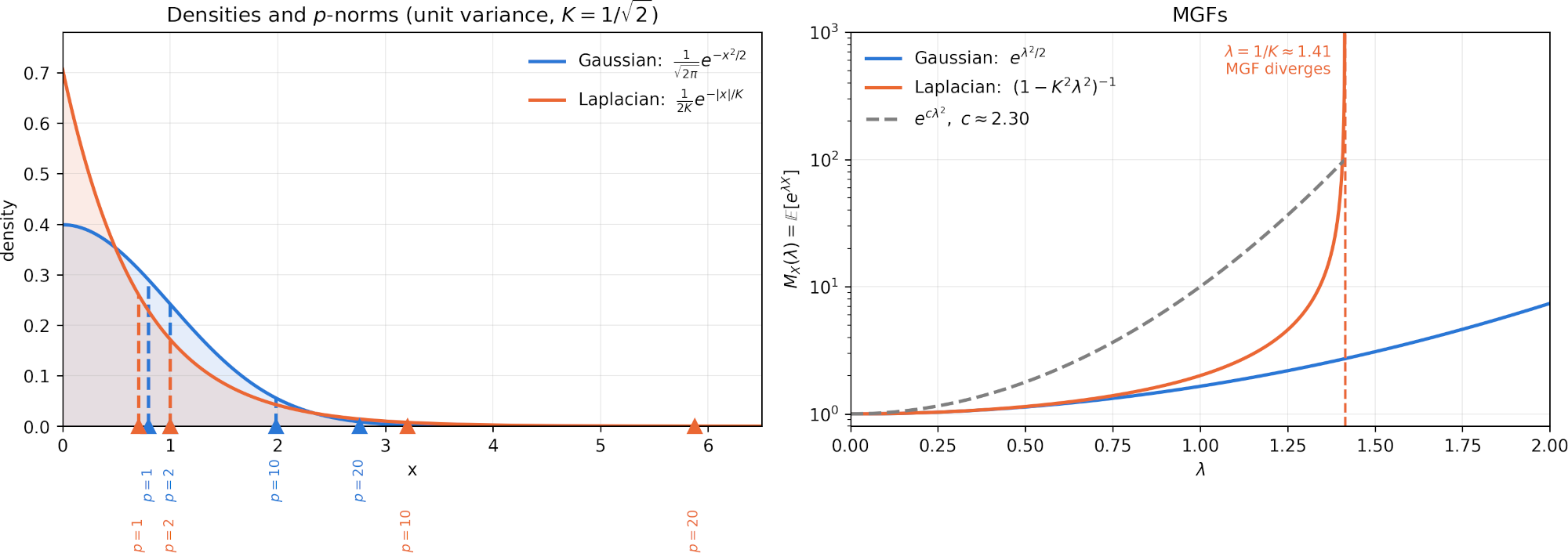
For $\alpha = 1$, the MGF is finite if and only if $\lambda < (eK)^{-1}$ (i.e. near the origin): In this case, we have $\kappa_p = (\lambda e K)^p$. This is a geometric series, which converges if and only if: $$ \lambda e K < 1 \iff \lambda < \frac{1}{eK} $$ Note that this bound is tight in the sense that exponential distributions (satisfying $\alpha=1$) have divergent MGFs. Consider the PDF $f(t) = K^{-1} e^{-t/K}$. Then, the MGF is: $$ \mathbb{E}[e^{\lambda X}] = \frac{1}{K} \int_0^\infty e^{\lambda t} e^{-t/K} dt = \frac{1}{K} \int_0^\infty e^{-(\frac{1}{K} - \lambda)t} dt $$ Clearly, the integral diverges when $\lambda \geq \tfrac{1}{K}$, which obeys (up to a constant) the condition given above.
For $\alpha < 1$: The MGF never exists. In this case, the exponent $1 - 1/\alpha$ is negative, and thus the denominator becomes a numerator $p^\nu$ for some positive $\nu$. The series $\sum_{p=0}^\infty (p^\nu \lambda e K)^p$ diverges for all $\lambda$.
So, as we see, not every sub-$\alpha$ distribution has a MGF for every $\lambda$. Subgaussian distributions sit comfortably in the fully convergent range, and exactly $\alpha=1$ distributions converge only for $\lambda \lesssim \tfrac{1}{K}$:
let us now find bounds for the $\alpha, \lambda$ cases where the MGF exists:
Let $X$ be a sub-$\alpha$ random variable ($\alpha \geq 1$), i.e. $\lVert X \rVert_p \leq K p^{\frac{1}{\alpha}}$. Expanding and bounding its MGF ($\lambda \geq 0$) yields the inequality: $$ M_X(\lambda) = 1 + \lambda \mathbb{E}[X] + \sum_{p=2}^\infty \frac{\lambda^p}{p!} \mathbb{E}[X^p] \leq 1 + \lambda \mathbb{E}[X] + \sum_{p=2}^\infty \frac{\lambda^p}{p!} \mathbb{E}[|X|^p] $$ Then, applying the sub-$\alpha$ bound and Stirling (as in the convergence analysis): $$ M_X(\lambda) \leq 1 + \lambda \mathbb{E}[X] + \sum_{p=2}^\infty \Big( \frac{\lambda e K}{p^{1 - 1/\alpha}} \Big)^p $$
Let’s now bound the $p \geq 2$ sum. Overall, the strategy will be to find the largest term inside of the sum, and argue that the whole (convergent) sum is of comparable size. We can bound $\kappa_p = (\lambda e K)^p / p^{p - p/\alpha}$ analytically if we treat $p$ as a real value and take the log-derivatives wrt $p$: $$ \begin{align*} f(p) = &\log(\kappa_p) = p \big[\log(\lambda e K) - (1 - 1 /\alpha)\log(p) \big] \\ \nabla_p f(p) = & p [0 - (1 - 1/\alpha) \underbrace{\nabla_p \log(p)}_{1/p}] + \log(\lambda e K) - (1 - 1/\alpha) \log(p) \\ = & \log(\lambda e K) - (1 - 1 / \alpha) (1 + \log(p)) \\ \nabla_p^2 f(p) = & 0 - (1 - 1 / \alpha) (0 + 1 / p) = - \frac{1 - 1 / \alpha}{p} \\ \nabla_p f(p_{\sharp}) = 0 \Rightarrow & \log(\lambda e K) = (1 - 1 / \alpha) (\underbrace{1 + \log(p_\sharp)}_{\log(ep_\sharp)}) \Rightarrow \lambda e K = (ep_\sharp)^{1 - 1 / \alpha} \\ \Rightarrow & p_\sharp = \frac{1}{e} (\lambda e K)^{\frac{\alpha}{\alpha - 1}} \\ f(p_\sharp) = & p_\sharp \big[\underbrace{\log(\lambda e K)}_{(1 - 1/\alpha) (1 + \log(p_\sharp))} - (1 - 1 /\alpha)\log(p_\sharp) \big] = (1 - 1/\alpha) p_\sharp \\ \Rightarrow \kappa_\sharp = &\exp(f(p_\sharp)) = \exp\Big(\frac{1 - 1/\alpha}{e} (\lambda e K)^{\frac{\alpha}{\alpha - 1}}\Big) \end{align*} $$ As with the convergence analysis, behaviour of this system depends on the value of $\alpha$, and clearly exposes why $\alpha=1$ is a tipping point:
In the case of $\alpha = 1$:
$~$
- $\nabla_p f(p)$ is constant, so $f(p)$ is linear, and thus the $\kappa_p$ terms in the sum grow/shrink geometrically. This is a geometric series that converges only if $|\lambda e K| < 1$.
- Convergent geometric series obey $\sum_{p=2}^\infty r^p = \tfrac{r^2}{1 - r}$. Taking some fixed $r = \lambda e K < 1$, we get convergence and $\mathcal{O}(\lambda^2 K^2)$ growth for $\lambda \in [0, r / eK]$. And since $1 + x \leq e^x$, we also have $M_X(\lambda) = \lambda \mathbb{E}[X] + \mathcal{O}(e^{\lambda^2 K^2})$ (useful later for Chernoff)
In the case of $\alpha > 1$:
$~$
- $\nabla_p^2 f(p) < 0$, so $f(p)$ is concave and thus the maximum $\kappa_\sharp$ always exists and is unique. Crucially, while this is true for every $\lambda$, the location of the peak $p_\sharp$ increases with $\lambda$
- Since $\kappa_p$ decays after $p_\sharp$, for any $m \geq p_\sharp$, the sum of all $\kappa_{p < m}$ can be upper-bounded as $m \kappa_\sharp$. And the $\kappa_{p\geq m}$ sum can also be upper-bounded to $c \kappa_\sharp$ for some constant $c$ via a convergent geometric series (see extra derivation below), resulting in the overall $(m + c) \kappa_\sharp$ bound for the sum. Replacing the definition of $\kappa_\sharp$, we get a growth of $(m + c) (\exp((1 - 1/\alpha) / e))^{(\lambda e K)^{\frac{\alpha}{\alpha - 1}}} = \mathcal{O}(\exp(C (\lambda K)^{\frac{\alpha}{\alpha - 1}}))$ (the constant $C$ in the exponent absorbs some terms)
- Note that, when $\alpha \geq 2$, this generic bound from above also obeys $\mathcal{O}(e^{C \lambda^2 K^2})$
To derive the convergence of the $\kappa_{p\geq m}$ sum, we pick a convenient cutting point satisfying $m \geq 2^{\frac{1}{1 - 1/\alpha}} e p_\sharp > p_\sharp$. In this case, we now show that $\kappa_{p + 1} \leq \tfrac{1}{2} \kappa_p$, so the sum is a convergent geometric series with decay ratio $1/2$, upper-bounded by $2 \kappa_\sharp$: $$ \frac{\kappa_{p + 1}}{\kappa_p} = \frac{(\lambda e K)^{p + 1}}{(\lambda e K)^{p}} \underbrace{\frac{p^{p - p/\alpha}}{(p + 1)^{(p + 1) - (p + 1)/\alpha}}}_{(p + 1)^{p - p/\alpha + (1 - 1/\alpha)}} = \frac{\lambda e K}{(p + 1)^{1 - 1/\alpha}} \underbrace{\Big( \frac{p}{p + 1} \Big)^{p - p/\alpha} }_{< 1} $$ Now replace $\lambda e K = (e p_\sharp)^{ 1- 1 /\alpha}$ via $p_\sharp$ definition in the numerator, and use $p + 1 > m \geq 2^{\frac{1}{1 - 1/\alpha}} e p_\sharp$ in the denominator, and the result follows: $$ \frac{\kappa_{p + 1}}{\kappa_p} < \Big( \frac{e p_\sharp}{m} \Big)^{ 1- 1 /\alpha} \leq \Big(2^{-\frac{1}{1 - 1/ \alpha}} \Big)^{ 1- 1 /\alpha} = \frac{1}{2} $$
Concluding the analysis:
As we have seen, the bounds of $M_X(\lambda)$ for sub-$\alpha$ distribution $X$ with scale parameter $K$ and $\alpha \geq 1$ are a bit involved, but can be characterized depending on $\alpha, \lambda$ in the following form $$ M_X(\lambda) = \lambda \mathbb{E}[X] + \mathcal{O}(\dots) $$ With the following remarks:
$~$
- If $\alpha=1$, then $\mathcal{O}(\exp(\lambda^2 K^2))$ for sufficiently small $\lambda$, and diverges otherwise
- If $\alpha > 1$, then $\mathcal{O}(\exp(C (\lambda K)^{\frac{\alpha}{\alpha - 1}}))$ for all $\lambda$. In particular, if $\alpha \geq 2$, the quadratic $\mathcal{O}(\exp(C \lambda^2 K^2))$ holds for all $\lambda$
A final remark: often we assume $X$ is centered, which allows us to get rid of the linear $\lambda \mathbb{E}[X]$ term and establish the $M_X(\lambda) = \mathcal{O}(\dots)$ bound. This works because centering does not affect the sub-$\alpha$ status of $X$. This can be shown via Jensen and Lyapunov’s inequalities ($|\mathbb{E}[X]| \leq \mathbb{E}[|X|] = \lVert X \rVert_1 \leq \lVert X \rVert_p$). The $p$-norm changes only by a constant factor: $$ \lVert X - \mathbb{E}[X] \rVert_p \leq \lVert X \rVert_p + \underbrace{ \lVert \mathbb{E}[X] \rVert_p}_{ | \mathbb{E}[X] |} \leq 2 \lVert X \rVert_p $$
Great! but what does this kind of growth exactly mean in terms of tail bounds? To derive the converse way, we can find the optimal $\lambda$ and apply Chernoff:
Let $X$ be a zero-mean random variable satisfying $M_X(\lambda) \leq \exp( C (\lambda K)^\beta )$ for $\beta > 1$ on its feasible range $\lambda \in [0, \lambda_{\text{max}}]$. Injecting this MGF bound into the Chernoff inequality and taking the logarithm yields: $$ \log P(X \geq t) \leq \underbrace{C(\lambda K)^\beta - \lambda t}_{f(\lambda)} $$ We then seek the tightest bound $\lambda_\sharp = \arg \min_{\lambda \in [0, \lambda_{\text{max}}]} f(\lambda)$. Differentiation shows that $f$ is convex with respect to $\lambda$ and $\lambda_\sharp$ is analytic:
$$ \begin{align*} \nabla_\lambda f(\lambda) = &CK^\beta \beta \lambda^{\beta - 1} - t \\ \nabla_\lambda^2 f(\lambda) = & CK^\beta \beta (\beta - 1) \lambda^{\beta - 2} > 0 \quad \text{(convex)} \\ \nabla_\lambda f(\lambda_\sharp) = 0 \Rightarrow &\lambda_\sharp^{\beta - 1} = \frac{t}{C \beta K^\beta } \Rightarrow \lambda_\sharp = \Big( \frac{t}{C\beta K^\beta}\Big)^{\frac{1}{\beta - 1}} \end{align*} $$ And all we need to do now is replace $\lambda$ with the optimal value in the Chernoff bound, to obtain a probability tail bound that depends only on $\beta, K, t$. But recall that $\lambda$ is constrained to the feasible range, and $\lambda_\sharp$ may fall outside! This induces a “branching” behaviour in the bound:
Case 1: $\lambda_\sharp \leq \lambda_{\text{max}}$ (optimal):
In this case, we can make use of the stationarity equality $CK^\beta \beta \lambda_\sharp^{\beta - 1} = t$, and $K^\beta = (K^{\beta-1})^{\frac{\beta}{\beta - 1}}$: $$ \begin{align*} C (\lambda_\sharp K)^\beta - \underbrace{\lambda_\sharp t}_{C\beta (\lambda_\sharp K)^\beta} = &C (\lambda_\sharp K)^\beta (1 - \beta) = C (1 - \beta) K^\beta \underbrace{ \Big(\frac{t}{C \beta K^\beta}\Big)^{\frac{\beta}{\beta - 1}} }_{ \lambda_\sharp^\beta}\\ = & -C (\beta - 1) \Big(\frac{t}{C \beta K}\Big)^{\frac{\beta}{\beta - 1}} = -\underbrace{\frac{C (\beta - 1)}{(C \beta)^{\frac{\beta}{\beta - 1}}}}_{\eta_1} \Big(\frac{t}{ K}\Big)^{\frac{\beta}{\beta - 1}} \end{align*} $$ Note that we kept $K$ out of the factored out constant $\eta_1$, since this is one parameter we also care about for the tail bounds. Also note that $t/K$ is affected by the exponent $\beta$, which means that smaller $\beta$ leads to tighter bounds.
Case 2: $\lambda_\sharp > \lambda_{\text{max}}$ (slack):
In this case we cannot pick $\lambda_\sharp$, since it is not feasible (e.g. the MGF for that value does not exist). What we can do is express $t_{\text{max}}$ as a function of $\lambda_{\text{max}}$, since $\lambda_\sharp$ grows with $t$:
$$ \lambda_\sharp > \lambda_{\text{max}} \Rightarrow \frac{t}{C\beta K^\beta} > \lambda_{\text{max}}^{\beta - 1} \Rightarrow t > \underbrace{C\beta K^\beta \lambda_{\text{max}}^{\beta - 1}}_{t_{\text{max}}} $$
Also, recall that $f(\lambda)$ is convex: this dictates that the best posible choice is the “closest” feasible one, i.e. whenever $t > t_{\text{max}}$, we use $\lambda_{\text{max}}$ for our Chernoff bound.
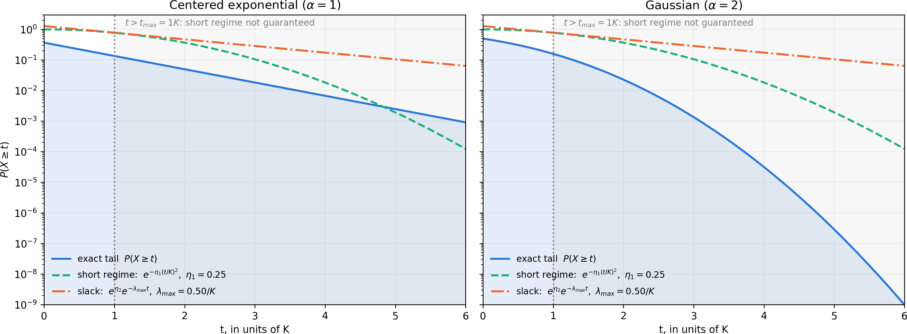
Unfortunately, as the $t > t_{\text{max}}$ gap widens, our bound at $\lambda_{\text{max}}$ gets more inefficient. This “slack” is reflected in one way: we cannot make use of stationarity. Instead, we crudely replace in log-Chernoff with $f(\lambda_{\text{max}})$ (no derivation): $$ \underbrace{C(\lambda_{\text{max}} K)^\beta}_{\eta_2} - \lambda_{\text{max}} t $$ We see that, in this inefficient regime, $t$ is not affected by the exponent $\beta$ due to our inability to inject $\lambda_\sharp$.
Putting everything together:
The above branching analysis splits the behaviour of Chernoff in 2 clear regimes (optimal/slack), but it still doesn’t directly answer the question: What are the corresponding tail bounds in terms of $(\alpha, K, t)$, and which one applies where?
Let’s go case by case:
$~$
-
Every $\beta\leq 2$ satisfies $\log M_X(\lambda) = \mathcal{O}(\lambda^2 K^2)$, yielding the following subgaussian tail bounds: $$ P(|X| \geq t) \underbrace{\leq 2 P(X \geq t)}_{\text{union bound}} \leq 2 \exp \Big( - \eta_1 \Big(\frac{t}{K} \Big)^2 \Big) $$
-
Note that, if we set $\alpha = \tfrac{\beta}{\beta - 1}$ (conversely, $\beta = \tfrac{\alpha}{\alpha - 1}$), the above $\beta \leq 2$ is satisfied for every $\alpha \geq 2$. But we also know that $\log M_X(\lambda) = \mathcal{O}(\lambda^2 K^2)$ is satisfied for all $\alpha \geq 1$ (and thus for all $\beta \geq 1$) with $\lambda_{\text{max}} \lesssim \tfrac{1}{K}$ (i.e. $t_{\text{max}} \lesssim C \beta K$). In all those cases, the above subgaussian tail applies
-
More generally, for any $\alpha > 1$ we saw that $\lambda_{\text{max}}$ is unbounded (this corresponds to any bounded $\beta$). In all those cases and for all $t$, the optimal (case 1) tail bound applies (but it may not be the tightest): $$ P(|X| \geq t) \leq 2 \exp \Big( - \eta_1 \Big(\frac{t}{K} \Big)^{\alpha} \Big) $$
-
Finally, if $\alpha = 1$, we know that $\lambda_{\text{max}} \lesssim 1 / K$ (i.e. $t_{\text{max}} \lesssim C \beta K$). The $t > t_{\text{max}}$ regime for $\alpha = 1$ is the only instance where we must resort to the slack (case 2) bound, revealing its subexponential nature: $$ P(|X| \geq t) \leq 2 e^{\eta_2} e^{-\lambda_{\text{max}} t} $$
Thus we have covered all cases. The TLDR is that, if $X$ is a centered RV satisfying $M_X(\lambda) \leq \exp( C (\lambda K)^\beta )$ for $\beta > 1$, the subgaussian bound always applies for $t \leq t_{\text{max}}$, and above that threshold, the subexponential bound is forced if $\alpha=1$, otherwise the “efficient” bound also applies with corresponding $\alpha$ exponent.
With this deeper understanding of the MGF for sub-$\alpha$ distributions, we are finally equipped to derive some popular and useful concentration inequalities applied to sums of independent, centered random variables.
Tail bounds for sums of independent random variables
We first introduce the general mechanism to obtain such bounds, which goes as follows:
- Given are $X_1, \dots, X_n$ sub-$\alpha$ independent and centered random variables with individual scale parameters $K_i$
- For each such $X_i$, get the corresponding MGF bound
- Obtain the MGF of the sum, which under independence is the product of the individual MGFs
- This final MGF turns out to scale only by $\sqrt{n}$, and Chernoff applies as already discussed
Let’s do it!
Let $X_1, \dots, X_n$ be centered random variables, each satisfying a sub-$\alpha$ tail bound with scale parameter $K_i$. Let also $S = \sum_i^n X_i$ (and thus clearly $\mathbb{E}[S] = 0$). Then, for some $c > 0$ and $\lambda_{\text{max}}$, it holds:
$$ P(|S| > t) \leq 2 \exp \Big[ -c \min \Big( \frac{t^2}{\sum_i K_i^2}, \quad \lambda_{\text{max}} t \Big) \Big] $$
To show this, let’s start recalling the (convergent) MGF bounds for each individual $X_i$: $$ M_{X_i}(\lambda) \leq \exp(C \lambda^2 K_i^2) \text{ if } \begin{cases} \lambda \geq 0, \alpha \geq 2 \\ \lambda \leq \lambda_i^{\text{max}}, \alpha \geq 1 \end{cases} $$ Furthermore, recall that the MGF of an independent sum is the product of the individual MGFs. This allows us to bound $M_S(\lambda)$ (for the above cases where the MGF exists): $$ \begin{align*} M_S(\lambda) = &M_{\sum_i^n X_i}(\lambda) = \prod_i^n M_{X_i}(\lambda) \leq \prod_i^n \exp(C \lambda^2 K_i^2) \\ \Rightarrow M_S(\lambda) \leq &\exp( \sum_i^n C \lambda^2 K_i^2) = \exp(C \lambda^2 \underbrace{\sum_i^n K_i^2}_{K_S^2}) \end{align*} $$ So we see that $M_S(\lambda)$ satisfies a bound in the form $\mathcal{O}(\exp(C (\lambda K_S)^2))$. Furthermore, we see that $K_S = \sqrt{\sum_i K_i}$, confirming that the scale of the sum grows with $\sqrt{n}$ (this is only true under independence). We can now apply Chernoff, as derived in the previous section, to obtain the corresponding probability tail bounds:
In the optimal regime, where this MGF is supported, the quadratic log-MGF yields the efficient (subgaussian) bound: $$ P(|S| > t) \leq 2 \exp(-\eta_1 (t / K_S)^2) $$ In the slack regime, where the MGF is unbounded, we take the closest feasible parametrization, which we defined to be $\lambda_{\text{max}}$, and we get $$ P(|S| > t) \leq 2 \exp(\eta_2 - \lambda_{\text{max}} t) $$
In practice, we pick whichever is tighter (we also derived a $t_{\text{max}}$ above which the slack regime is triggered). Absorbing the $\eta_1, \eta_2$ constants into $c$ yields the result.
With this, we can now derive the Hoeffding and Bernstein inequalities as particular instances of this general mechanism:
Let $X_1, \dots, X_n$ be independent, centered and subgaussian ($\alpha = 2$) variables with scales $K_i$. In this case, we have $\lambda_{\text{max}} = \infty$, since $\alpha = 2$ implies that every individual MGF converges for all $\lambda$. Therefore, the slack regime never triggers, and we get: $$ P \Big( \Big| \sum_i^n X_i \Big| \geq t \Big) \leq 2 \exp \Big( - c \frac{t^2}{\sum_i^n K_i^2} \Big) $$ Main takeaways:
$~$
- Sums of independent, centered subgaussians are subgaussian
- Scale grows with $\sqrt{\sum_i K_i^2}$. Crucially, the scale of the average between $n$ variables of same-scale $K$ shrinks with $K/\sqrt{n}$ (hence high-dimensional averages concentrate sharply)
Let $X_1, \dots, X_n$ be independent, centered and subexponential ($\alpha = 1$) variables with scales $K_i$. Recall that in this case MGF convergence can only be guaranteed for $\lambda \leq \lambda_{\text{max}}$, where it grows quadratically, and thus we have: $$ \begin{align*} \lambda_{\text{max}} = &\min_i \lambda_{\text{max}_i} \lesssim \min_i \frac{1}{K_i} = \frac{1}{\max_i K_i} \\ t_{\text{max}} \lesssim & C (\sum_i K_i^2) \lambda_{\text{max}} \asymp \frac{\sum_i^n K_i^2}{\max_i K_i} \text{ (for some constant $C$)} \end{align*} $$
As a consequence, the “slack” branch is activated for all $t \geq t_{\text{max}}$, and both branches survive: $$ P \Big( \Big| \sum_i^n X_i \Big| \geq t \Big) \leq 2 \exp \Big( - c \min \Big( \frac{t^2}{\sum_i^n K_i^2}, \quad \underbrace{\frac{1}{\max_i K_i} t}_{\text{active for } t > t_{\text{max}}} \Big) \Big) $$
Main takeaways:
$~$
- Moderate deviations ($t \leq t_{\text{max}}$) still obey the subgaussian bound: many small deviations are present and cancel each other effectively
- Large exponential deviations are dominated by $\max_i K_i$: averaging does not dampen single heavy summands fast enough, which is exactly why the MGF diverges in those regimes
Out of bounds section
Hopefully this post manages to be a low-friction way to cover some of these wonderful and powerful bits on concentration bounds. Of course, there is much more content and rigor out there (which avoids the completely unnecessary and inappropriate jokes pertaining –but not limited to– grower-vs-shower moments, the hidden limitations of alphas with fat tails, and how your $p$ looks like if you bound your tail). The standard reference is, as mentioned at the beginning:
High-Dimensional Probability: An Introduction with Applications in Data Science – Roman Vershynin (Cambridge University Press, 2018 – 2nd ed. 2026)
And suggestions for improvement are always welcome. A few follow-ups that I’d love to incorporate at some point in the future:
- Further discussion on Orlicz norms
- Better discussion on constants
- The in-between regime of “efficient” Chernoff for $\alpha > 1$
- Connections to Johnson-Lindenstrauss and the Restricted Isometry Property
- Further concentration bounds, such as noncommutative Bernstein and Hanson-Wright
- Applications in randomized linear algebra (Ethan Epperly has this one pretty well covered, I also wrote this other post on diagonal estimation)