A Tour of the RIP
The Restricted Isometry Property (RIP) is a highly effective and straightforward way to guarantee that sparse recovery (a certain type of hard and useful inverse problem) can be solved efficiently. Understanding the mechanics behind those guarantees is a very good way to gain understanding of the main questions surrounding the RIP, such as:
$~$
- What is the RIP, and motivations behind it
- Why is the RIP sufficient for exact and unique sparse recovery
- Why random matrices satisfy the RIP with high probability for $n \ll N$
- Measurement bounds: relations between $n$, $N$ and sparsity $k$
The aim of this post is to provide the minimal amount of machinery that can cover the above points, articulated as a linear and easy-to-follow sequence of results: While the overall structure is kept intentionally minimal, the step-by-step derivations are more exhaustive and don’t skip many “trivial” steps. The more rigorous and strictly necessary references can be reduced to these 2 short seminal papers:
- Sparse Representation of a Polytope and Recovery of Sparse Signals and Low-rank Matrices (Cai & Zhang, 2013) [CZ13]
- A Simple Proof of the Restricted Isometry Property for Random Matrices (Baraniuk et al. 2006) [BDDW08]
Skip to the green boxes for the step-by-step derivations of their main results.
Compressed Sensing and the RIP
Consider the inverse problem of recovering a sparse vector $\dot x$ (i.e. many of its entries are zero) from highly incomplete linear measurements ($n \ll N$): $$ y = \Phi \dot x, \quad \Phi \in \mathbb{R}^{n \times N} $$
This is a relevant setting, since sparse $\dot x$ appear in many problems of interest, and measurements can be costly (the classical example is MRI scans). Unfortunately, this is an underconstrained problem and admits infinitely many solutions, exposed to large errors.
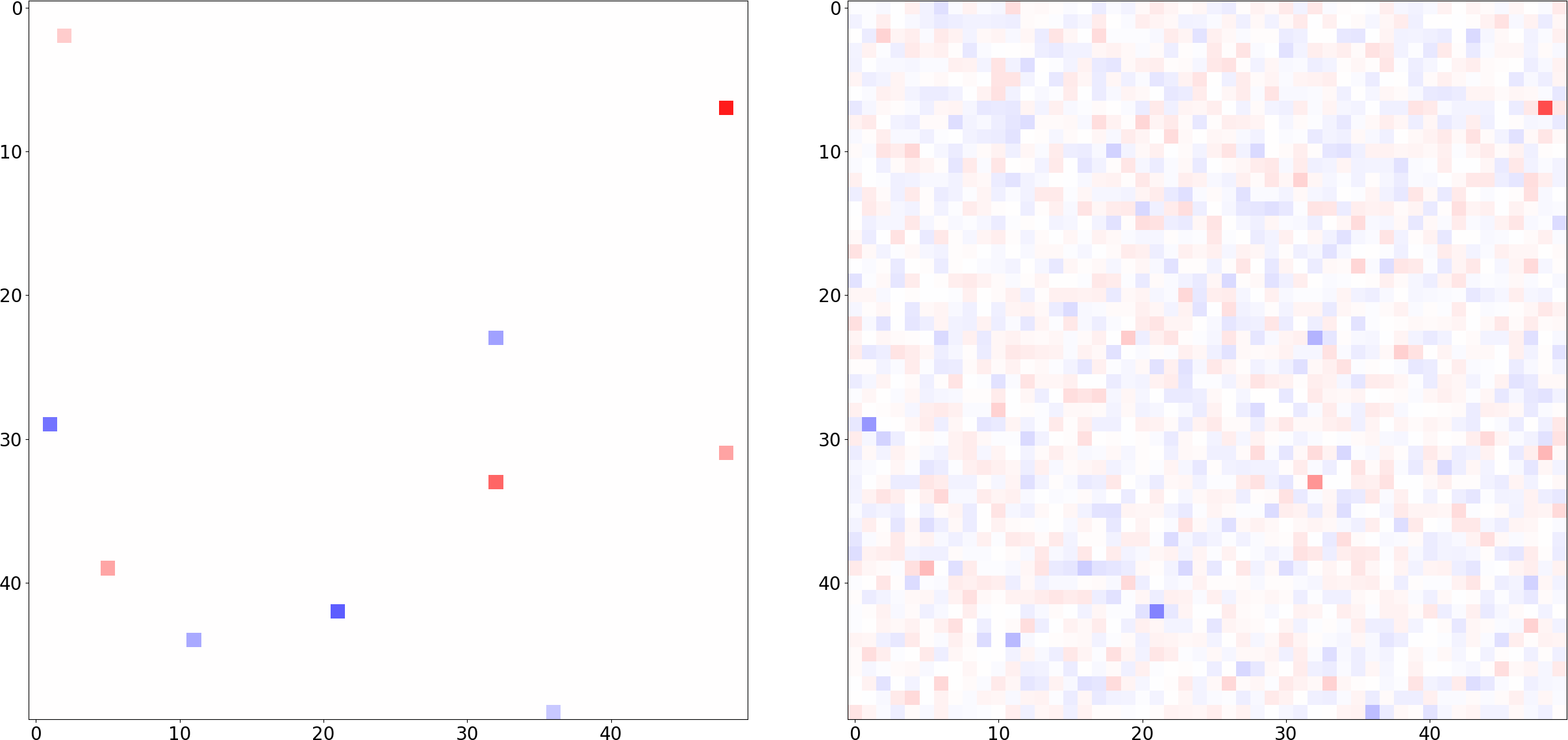
The advantage in this case is that we know $\dot x$ is sparse, so among all possible solutions (such as the 2 images above), we only care about the sparsest one (such as the left one): $$ \hat x \quad = \quad \operatorname*{argmin}_{x} \quad \lVert x \rVert_0 \quad s.t. \quad y = \Phi x \qquad (P_0) $$
Unfortunately, $P_0$ is a combinatorial problem: Since we only know $(y, \Phi)$, finding the optimal position and value of $k$ nonzeros in $\dot x$ may require exploring all $\binom{N}{k}$ combinations. A major insight is that any sparse $\dot x$ can be recovered exactly and uniquely from $(y, \Phi)$ by solving the following “convex relaxation” $(P_1)$: $$ \hat x \quad = \quad \operatorname*{argmin}_{x} \quad \lVert x \rVert_1 \quad s.t. \quad y = \Phi x \qquad (P_1) $$ Crucially, $P_1$ is efficient and scalable: Practical guarantees for $n \ll N$ can be obtained, and first-order solvers (such as FISTA) can solve this problem with only $\mathcal{O}(nN)$ memory, yielding $\varepsilon$-optimal approximations after $1 / \sqrt{\varepsilon}$ iterations. But this sounds too good to be true: Are we really solving a combinatorial problem in polynomial time?
- The measurement matrix $\Phi$ needs to be “well behaved”. Not any $\Phi$ works
- $\dot x$ itself needs to be sufficiently sparse and $n$ needs to be “sufficiently large”
For this subset of problems, $P_0 \equiv P_1$ and a polynomial and exact recovery is indeed possible!
But what does “well behaved” and “sufficiently large $n$” mean more concretely? Initial work based on the coherence among the columns of $\Phi$ was able to provide exact recovery guarantees for $k$-sparse signals whenever $n \asymp k^2$, and also led to deterministic approaches to construct such $\Phi \in \mathbb{R}^{c k^2 \times N}$ (such as Equiangular Tight Frames and DeVore matrices). So yes, if we get to pick a nice $\Phi$, we do have a deterministic way to solve $P_0$ in polynomial time and memory.
But $k^2$ may be large, and we can in fact do better: One of the main reasons to focus on the Restricted Isometry Property (RIP) is that the RIP provides a very succinct and clear pathway to obtain strong recovery guarantees for only $n \asymp k \log(N / k)$ measurements, well below $k^2$. This is typically articulated as follows:
- The RIP is a sufficient condition for $P_0 \equiv P_1$
- Any subgaussian i.i.d. $\Phi$ with $n \asymp k \log(N / k)$ satisfies the RIP with very high probability
- Furthermore:
- The $n = \mathcal{O}(k \log(N / k))$ measurement regime is optimal for a robust/compressible recovery (this is related to Gelfand widths of $\ell_p$ balls, see 1.2. here for nuances and discussion)
- Since $\Phi$ is nonadaptive (i.e. obtained witout looking at any data), it is also universal, i.e. guarantees for $\Phi$ hold, as long as $x$ is sparse on some fixed orthonormal basis $\Psi$. This means that we can blindly use $y = \Phi \dots$ and $y$ will still have all the necessary information, we just need to know $\Psi$ at the time of solving $P_1$ (see Section 6 in [BDDW08])
- Verifying the RIP is NP-Hard for a given, arbitrary $\Phi$: We can only make RIPness statements if we know the structure of $\Phi$ (Gaussian, equiangular…)
- These results extend to broader settings such as noisy and nonuniform with little overhead. In particular, it also extends to low-rank matrix recovery: The measurement bound to recover $N \times N$ matrices of rank $k$ is $n \asymp Nk$, no log factor is needed (see here)
The main goal of this post is to provide a linear, direct and succinct way to understand points 1 and 2 with step-by-step proofs and references. The focus will be on the noiseless case, and references are intentionally concise. I apologize in advance for omitting many relevant works and results. Readers are also invited to read the links in point 3 for more details. Also note that the RIP is not the only—nor the most general—way to obtain recovery guarantees, see e.g. nullspace property, incoherence/isometry, and golfing schemes.
RIP as a sufficient condition for uniqueness and correctness of $P_1$
Let’s recall the setup: we obtained some measurements $y = \Phi \dot x \in \mathbb{R}^n$ where $(y, \Phi)$ are known, and $\dot x \in \mathbb{R}^N$ is assumed to be $k$-sparse. We then solve the convex problem: $$ \hat x \quad = \quad \operatorname*{argmin}_{x} \quad \lVert x \rVert_1 \quad s.t. \quad y = \Phi x \qquad (P_1) $$
The aim is to isolate sufficient conditions under which $\hat x = \dot x$. In this section we will see that, if $\Phi$ satisfies the following RIP with $\delta_{2k} < 1 / \sqrt{2}$, then $\hat x$ is unique and correct, i.e. $\hat x =\dot x$, and there is no other $k$-sparse candidate anywhere in the feasible set:
But wait: didn’t we care about uniqueness and correctness of $P_1$? Why are we now defining an $\ell_2^2$ property, that applies to an $\ell_0$ constraint? This is one of the beauties of the RIP: the interplay between $\ell_0, \ell_1$ and $\ell_2$ may look all over the place, but is precisely what will allow us to apply strong results from linear algebra and random matrix theory directly to our sparse recovery problem down the line.
To showcase this, let’s start by showing that there cannot be a sparser candidate than $\hat x$. This is very straightforward to show with the RIP:
It now remains to show that $\hat x$ is not only sparsest, but also equal to $\dot x$ (i.e. we need to discard that there are two distinct, feasible, $2k$-sparse vectors). We will largely follow the Theorem 1.1 proof from [CZ13] and also borrow from [Candès, 2008]. The latter is a very succinct 4-page paper with a nice proof, but the former introduces relevant components that make the proof sharp and more general. We start by assuming the obtained $\hat x$ has an alias, i.e. there is another candidate $\hat x + h$ satisfying:
- $\Phi h = 0$ (both $\hat x$ and the alias are feasible)
- $\lVert \hat x \rVert_1 \geq \lVert \hat x + h \rVert_1$ (alias is at least as good in $\ell_1$ terms)
And the goal is to show that $h=0$ under RIP with $\delta_{2k} < 1 / \sqrt{2}$, i.e. such an alias cannot exist. Note that the RIP does not directly apply to this alias since here we don’t assume that $x + h$ is $k$-sparse. In order to navigate the trickier relationship between $\ell_1$ and $\ell_0$, we will make use of the following results:
Given any matrix $Z$, convex weights $\lambda_i\ge0$ with $\sum_i\lambda_i=1$, and any scalar $c$, define the weighted mean $\bar z=\sum_i\lambda_i z_i$. Then, $$ \sum_i \lambda_i \lVert \bar z - c z_i \rVert_2^2 + (1 - 2c) \sum_i \sum_{j > i} \lambda_i \lambda_j \lVert z_i - z_j \rVert_2^2 = (1 - c^2) \sum_i \lambda_i \lVert z_i \rVert_2^2 $$
For $c = 1/2$, it simplifies to: $$ \sum_i \lambda_i \lVert \bar z - \frac{1}{2} z_i \rVert_2^2 = \frac{1}{4} \sum_i \lambda_i \lVert z_i \rVert_2^2 $$
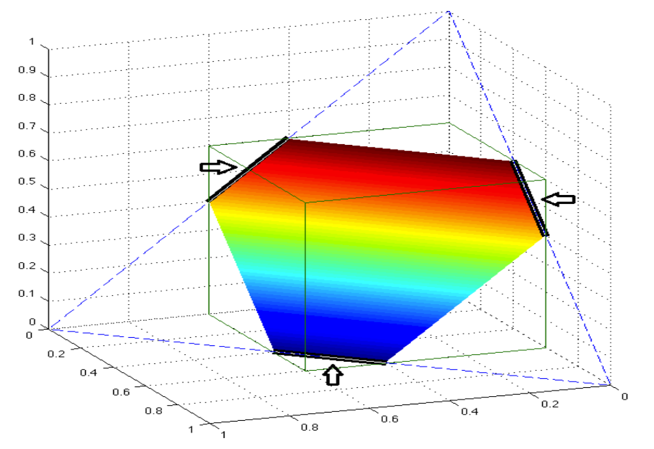
We will also need the following definitions and results:
- $S$ as the support of $\dot x$ (i.e. the $k$ entries where $\dot x$ is not zero). Also partition $h$ into its in-support and out-of-support components: $h = h_S + h_{\bar S}$.
- Cone constraint: $\lVert h_{S} \rVert_1 \geq \lVert h_{\bar S} \rVert_1$, because $\lVert \dot x \rVert_1 \geq \lVert \dot x + h \rVert_1 = \lVert \dot x + h_{S} \rVert_1 + \lVert h_{\bar S} \rVert_1 \geq \lVert \dot x \rVert_1 - \lVert \dot h_S \rVert_1 + \lVert h_{\bar S} \rVert_1$
- Jensen’s inequality: $\lVert \sum_i \lambda_i v_i \rVert_2^2 \leq \sum_i \lambda_i \lVert v_i \rVert_2^2$ (positive $\lambda_i$ adding to 1)
- Cauchy-Schwarz: $\lVert v \rVert_1 = \langle 1, v \rangle \leq \lVert 1 \rVert_2 \lVert v \rVert_2$
- Norm bound for $k$-sparse vectors: $\lVert v \rVert_2^2 \leq k \lVert v \rVert_\infty^2 \leq k \lVert v \rVert_1^2$
Set $\alpha = \lVert h_S \rVert_1 / k$ and partition $h_{\bar S} = h_\uparrow + h_\downarrow$, where $h_\uparrow$ contains all $h_{\bar S}$ entries greater than $\alpha$, and $h_\downarrow$ all the other entries. Then, $h_\uparrow$ is at most $k$-sparse (can’t have more than $k$ entries larger than $\alpha$), and $h_\downarrow$ is in the polytope $T(\alpha, s)$ with $\ell_0$ bound $\alpha$ (by definition) and $\ell_1$ bound $s\alpha = (k - \lVert h_\uparrow \rVert_0)\alpha$, since the cone constraint gives: $$ \lVert h_\downarrow \rVert_1 = \lVert h_{\bar S} \rVert_1 - \lVert h_\uparrow \rVert_1 \leq \underbrace{\lVert h_{S} \rVert_1}_{= k \alpha} - \underbrace{\lVert h_\uparrow \rVert_1}_{\geq \lVert h_{\uparrow} \rVert_0 \alpha} \leq \underbrace{(k - \lVert h_\uparrow \rVert_0)}_{s} \alpha $$
With this, we can now bound the $\ell_2^2$ norm of $h_\downarrow \in T(\alpha, s)$, since polytope elements can be expressed as a convex sum of $s$-sparse, $\alpha$-bounded vectors: $$ \begin{align*} \lVert h_\downarrow \rVert_2^2 &\leq \sum_i \lambda_i \lVert u_i\rVert_2^2 \leq \max_i \lVert u_i \rVert_2^2 \leq s \alpha^2 \leq k \alpha^2 = \Big(\frac{\lVert h_S\rVert_1}{\sqrt{k}}\Big)^2 \\ &\leq \lVert h_S \rVert_2^2 \leq \lVert h_S + h_\uparrow \rVert_2^2 = \lVert w \rVert_2^2 \end{align*} $$
This is good: $w = h_S + h_\uparrow$ is $2k$-sparse, and its $\ell_2$ norm dominates all other entries in $h$. Therefore, if we can show that $\lVert w \rVert_2^2 = 0$, then the whole $h$ must be 0 and thus $\hat x = \dot x$: $$ \lVert w \rVert_2^2 = 0 \Rightarrow h_\downarrow=0 \Rightarrow h = w + h_\downarrow = 0 $$ But how do we find the conditions that give $w=0$? Like in the previous green block, we want a result that looks something like $0 \leq f_\delta \lVert w \rVert_2^2$, so we know that $w=0$ whenever $f_\delta < 0$. Unfortunately, we cannot leverage the feasibility constraint $\Phi h = 0 \Rightarrow \Phi w = - \Phi h_\downarrow$, since the RIP does not apply to $h_\downarrow$. Also, applying the RIP on a generic $w$ is vacuous: $$ (1 - \delta) \lVert w \rVert_2^2 \leq \lVert \Phi w \rVert_2^2 \leq (1 + \delta) \lVert w \rVert_2^2 \Rightarrow (1 - \delta) \leq (1 + \delta) $$ The plan is to find two vectors that depend on $w$, are both $2k$-sparse and have different norm. Then, we can apply the RIP to both of them, putting the bigger on the left and the smaller on the right, leaving a nonzero gap in which the only solution is that everything is 0 via $w=0$. This is often called the “RIP squeeze” step.
To achieve this, we go back to the polytope satisfying the convex sum $h_\downarrow = \sum_i \lambda_i u_i$, and construct the vectors $z_i = w + \mu u_i$, for some constant $\mu \in (0, 1)$. This construction allows us to smuggle $h$ inside sparse vectors (last line given by the parallelogram identity): $$ \begin{align*} \bar z = &\sum_i \lambda_i z_i = w + \mu h_\downarrow = w + \mu h - \mu w = (1 - \mu) w + \mu h \\ \bar z - \frac{1}{2} z_i = &[(1 - \mu) w + \mu h] - \frac{w + \mu u_i}{2} = \underbrace{(\frac{1}{2} - \mu) w - \frac{\mu}{2} u_i}_{z_i’ \text{, $2k$-sparse}} + \mu h \\ &\sum_i \lambda_i \lVert \underbrace{ \Phi (\bar z - \frac{1}{2} z_i)}_{= \Phi \bar z_i’} \rVert_2^2 = \frac{1}{4} \sum_i \lambda_i \lVert \Phi z_i \rVert_2^2 \end{align*} $$
Note that these properties are true for all $\mu \in (0, 1)$. This will be useful later. Furthermore,
$~$
- All linear combinations of $w$ and $u_i$ are $2k$-sparse, since $w$ has $2k-s$ nonzeros, and each $u_i$ has $s$ nonzeros, so the RIP applies to all $z_i$ (right-hand side of the parallelogram identity)
- The $h$ component vanishes under $\Phi$, so the RIP also applies to the left-hand side of the parallelogram identity using $z_i'$
- Crucially, $z_i’$ is missing the $h$ component: Wrapping the last identity with the RIP creates a discrepancy between different norms on the signal domain and equal norms under the image of $\Phi$. We put the “smaller” one on the right to force the “squeeze”:
$$ \frac{1 - \delta_{2k}}{4} \sum_i \lambda_i \lVert z_i \rVert_2^2 \leq \frac{1}{4} \sum_i \lambda_i \lVert \Phi z_i \rVert_2^2 = \sum_i \lambda_i \lVert \Phi z_i’ \rVert_2^2 \leq (1 + \delta_{2k}) \sum_i \lambda_i \lVert z_i’ \rVert_2^2 $$ Expanding, and simplifying with $\sum_i \lambda_i \lVert u_i \rVert_2^2 = \xi^2 \leq \lVert w \rVert_2^2$ (from the previous chain of inequalities) and $(1/2 - \mu)^2 - 1/4 = \mu^2 - \mu$, we can expose the squeeze:
$$ \begin{align*} &\frac{1 - \delta_{2k}}{4} \sum_i \lambda_i \Big[ \lVert w \rVert_2^2 + \mu^2 \lVert u_i \rVert_2^2 \Big] \leq (1+\delta_{2k}) \sum_i \lambda_i \Big[ \Big(\frac{1}{2}-\mu \Big)^2 \lVert w \rVert_2^2 + \frac{\mu^2}{4} \lVert u_i \rVert_2^2 \Big] \\ &\Longrightarrow \frac{1 - \delta_{2k}}{4} (\lVert w \rVert_2^2 + \mu^2 \xi^2 ) \leq (1+\delta_{2k}) \Big[ \Big(\frac{1}{2}-\mu \Big)^2 \lVert w \rVert_2^2 + \frac{\mu^2}{4} \xi^2 \Big] \\ &\Longrightarrow \frac{1 - \delta_{2k}}{4} \lVert w \rVert_2^2 \leq (1+\delta_{2k}) (\mu^2 - \mu + 1/4) \lVert w \rVert_2^2 + \delta_{2k} \frac{\mu^2}{2} \underbrace{\xi^2}_{\leq \lVert w \rVert_2^2} \\ &\Longrightarrow 0 \leq \big[ (1+\delta_{2k}) (4\mu^2 - 4\mu + 1) + 2 \delta_{2k} \mu^2 - (1 - \delta_{2k}) \big] \lVert w \rVert_2^2 \\ &\Longrightarrow 0 \leq \big[ 2 (\underbrace{\mu^2 - \mu}_{\leq 0}) + \delta_{2k} (\underbrace{3 \mu^2 - 2 \mu + 1}_{> 0}) \big] \lVert w \rVert_2^2 \quad \text{(recall that $\mu \in (0, 1)$)} \end{align*} $$ We can see now that this inequality is now nonvacuous: $\lVert w \rVert_2^2 = 0$ is forced if the square brackets are negative, and this is guaranteed for every $\delta_{2k} < (2 (\mu - \mu^2)) / (3 \mu^2 - 2 \mu + 1)$. And since we are free to pick $\mu$ (this is a nuisance parameter we introduced, and the derivations hold for all $\mu \in (0, 1)$), we seek the value of $\mu$ that maximizes this ratio: $$ \begin{equation*} \max_{\mu \in (0, 1)} \frac{2(\mu - \mu^2)}{3 \mu^2 - 2\mu + 1} = \frac{1}{\sqrt{2}} \qquad \text{(achieved at $\mu=\sqrt{2} - 1$)} \end{equation*} $$ Thus, if we reproduce the above RIP squeeze with $\mu=\sqrt{2}-1$, any $\delta_{2k} < \frac{1}{\sqrt{2}}$ will force $\lVert w \rVert_2^2 = 0 \Rightarrow \lVert h \rVert_2^2 = 0 \Rightarrow \hat x = \dot x$, concluding that the $\ell_1$ recovery is unique and correct.
Addendum: to maximize the ratio, note that setting its derivative to 0 yields a quadratic equation (using $f$ as the numerator and $g$ as the denominator): $$ \nabla_\mu = \frac{f’ g - g’ f}{g’’} = 0 \Rightarrow f’g = g’f \Rightarrow \mu^2 + 2 \mu - 1 = 0. $$ Wth the only positive solution at the established $\mu = \sqrt{2} - 1$. Replacing in the ratio and using $\mu^2 = 1 - 2\mu$ yields the bound for $\delta$: $$ \frac{2(\mu - \mu^2)}{3 \mu^2 - 2\mu + 1} = \frac{6\mu - 2}{4 - 8 \mu} = \frac{6 \sqrt{2} - 8}{12 - 8\sqrt{2}} = \frac{1}{\sqrt{2}} \frac{6 \sqrt{2} - 8}{12/\sqrt{2} - 8} = \frac{1}{\sqrt{2}} $$
Recap: how did we just prove uniqueness and correctness under RIP?
- We defined and decomposed an $\ell_1$ alias $\hat x + h = \hat x + h_S + h_\uparrow + h_\downarrow$
- Via polytope covexity plus a few standard inequalities, we saw that $h_\downarrow$ is $\ell_2$-bounded by $w = h_S + h_\uparrow$. This is important because $w$ is $2k$-sparse, and $w=0$ means there is no alias
- We then found 2 different families of vectors that, once $\Phi$ is applied, have the same norm and are $2k$-sparse. This allows us to apply the “RIP squeeze”
- The RIP squeeze exposed a gap in $\ell_2$ that is unavoidable for $\delta_{2k} < 1 / \sqrt{2}$, unless $w=0$. This means that, for those $\delta$, a $2k$-sparse alias cannot exist
- So, under RIP with $\delta_{2k} < 1 / \sqrt{2}$, the $P_1$ solution is unique, sparsest (as shown in the previous block), and therefore correct.
Uniqueness and correctness under RIP: further results
The [CZ13] paper has a few other relevant results worth mentioning:
- The $\delta_{2k} < 1 / \sqrt{2}$ bound is tight: In Theorem 2.2, they construct a $\Phi$ with $\delta_{2k} = \tfrac{1}{\sqrt2} + \varepsilon$, for which there exists a feasible, non-sparse solution with lower $\ell_1$ norm (i.e. an alias), thus correctness and uniqueness cannot be guaranteed via RIP outside of this bound. Note that this is an adversarially constructed $\Phi$, but still exposes the tightness (think: an alias can exist)
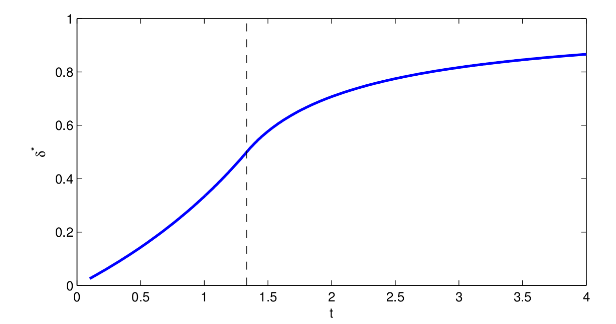
- The authors also provide optimal isometry constant for sparsity levels other than $2k$ (Theorem 1.1): For any $t \geq 4/3$, guarantees are given by $\delta_{tk} < \sqrt{\tfrac{t - 1}{t}}$ (see image below). They also proved the $\delta_k < 1/3$ bound in this other paper. This is a very useful result, since sometimes we can afford a tighter $\delta$ and thus the RIP only needs to hold for a smaller subset of sparse signals
- Results extend to stable recovery in the noisy scenario (Remark 2.1): We have derived the noiseless scenario directly, but the paper more generally proves that recovery under noisy measurements $y = \Phi \dot x + \eta$ (for some noise $\eta$) and model mismatch ($\dot x$ not exactly $k$-sparse) is linearly bounded by the noise/mismatch. Specifically, solving the Second-Order Cone Program $\hat x = \arg \min_x \lVert x \rVert_1 s.t. \lVert y - \Phi x \rVert_2 \leq \lVert \eta \rVert_2$ is error-bounded by $\lVert \dot x - \hat x \rVert_2 = \mathcal{O}(\lVert \eta \rVert_2) + \mathcal{O}(\tfrac{1}{\sqrt{k}} \lVert \dot x - \dot x_{\text{top-}k} \rVert_1)$, where $\dot x_{\text{top-}k}$ contains the $k$-largest entries of $\dot x$
- All results extend to the matrix case: The RIP bounds for (robust) recovery discussed so far also extend to the case of recovering a rank-minimal matrix subject to linear measurements via nuclear norm minimization (see this paper and the result below)
Before moving onto which $\Phi$ have the RIP, let me elaborate just a bit on the rank-minimization case:
Let’s start by defining the rank-RIP: We say that a linear operator $\mathcal{A}: \mathbb{R}^{N\times M} \to \mathbb{R}^q$ satisfies the rank-RIP with isometry constant $\delta_s \in [0, 1]$ if the following holds for all $\dot X \in \mathbb{R}^{N \times M}$ of rank $s$ or less: $$ (1 - \delta_s) \lVert \dot X \rVert_F^2 \leq \lVert \mathcal{A}(\dot X) \rVert_2^2 \leq (1 + \delta_s) \lVert \dot X \rVert_2^2 $$ Then, given $\dot X$ of rank $k$ and measurements $\mathcal{A}(\dot X) = b$, we solve the convex program: $$ \hat X = \arg \min_X \lVert X \rVert_* \text{ s.t. } \mathcal{A}(X) = b $$ And the results mentioned above translate one-to-one, namely, if $\mathcal{A}$ satisfies the rank-RIP with any of: $$ \begin{align*} \delta_k < \frac{1}{3}, \quad \text{or} \quad \delta_{tk} < \sqrt{\frac{t - 1}{t}}, \text{ } t \geq \frac{4}{3} \end{align*} $$
Then, $\hat X = \dot X$, and the recovery is unique and exact.
Subgaussian Random Matrices satisfy the RIP with $n \asymp k \log(N / k)$
As we briefly discussed in the introduction, certifying a particular RIP constant $\delta_s$ for a given arbitrary $\Phi$ turns out to be NP-Hard: in the worst case, we need to measure the isometry for all $\binom{N}{s}$ combinations of columns. Instead, we need an a-priori method that reliably generates RIP-friendly matrices.
- Deterministic methods exist, but they are affected by a near-quadratic measurement bottleneck, e.g. coherence matrices (Th. 3.1) require $n \asymp \tfrac{k^2}{\delta^2} \frac{\log^2(N)}{\log^2{k}}$ measurements to be $\delta$-RIP, and additive-combinatoric matrices (Th. 1) slightly break this bound, requiring $n \asymp k^{2 - \varepsilon_0}$ for a small constant $\varepsilon_0$ and $\delta = n^{-\varepsilon_0}$.
- In contrast, Randomized methods exhibit much better measurement bounds: $n \asymp \tfrac{k}{\delta^2} \log(N / k)$, at the cost of giving up deterministic guarantees: RIP is satisfied with overwhelming probability instead. A canonical citation for this result is the already mentioned [Candès & Tao, 2004]. Note: There is only one “coin flip”: Once we sample $\Phi$, either it satisfies the RIP or it doesn’t. If it does (which we can’t certify efficiently), recovery is guaranteed, there is no randomness involved in the correctness/uniqueness of $P_1$ under RIP (see the [CZ13] derivation in the previous section)
While deterministic RIP constructions are quite interesting and exciting, we focus here on the randomized case, which is the most commonly seen in practice due to its superior bounds and practical guarantees. There is a lot of great work covering the RIP for random matrices. Here we follow the “covering set” approach from [BDDW08], which is quite popular for being succinct (section 5 is less than 2 pages), insightful and powerful: it applies to any matrix with subgaussian, independent, zero-mean entries.
The main 2 ingredients are the tail probability bounds of a random varialble, and the cardinality of a covering set:
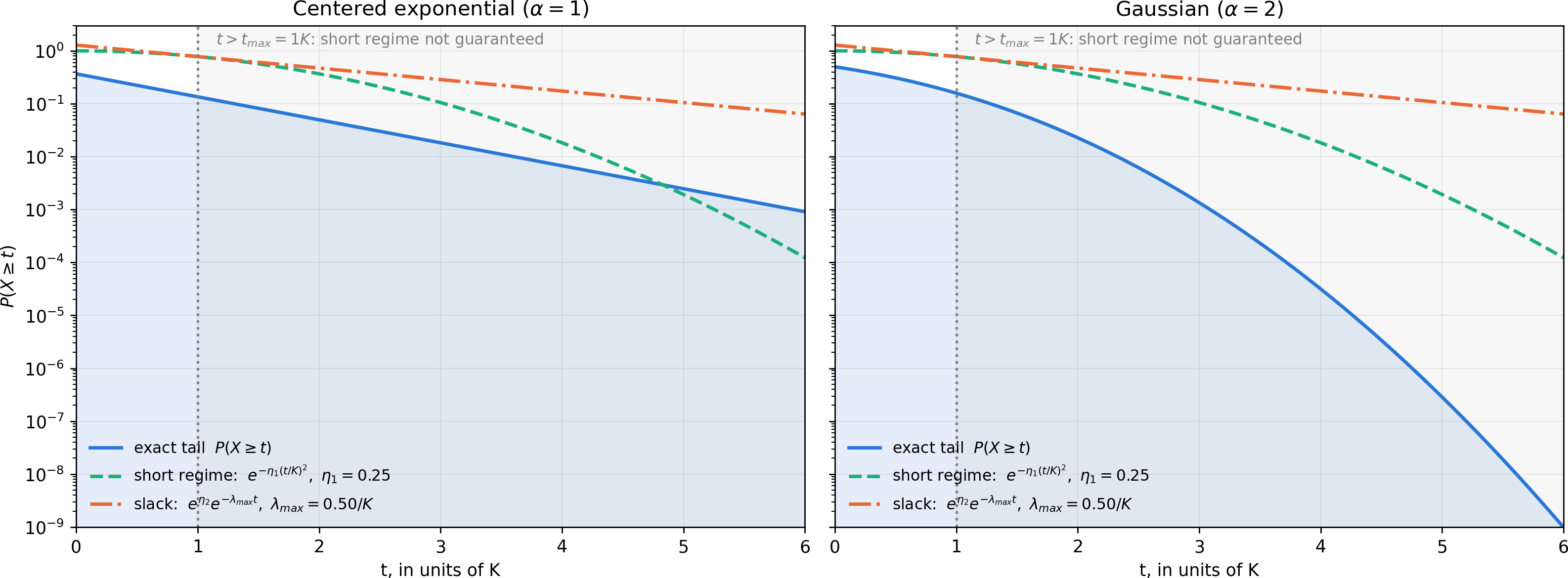
We say that a real-valued random variable $X$ has sub-$\alpha$ tail bounds with scale parameter $K$ if, for all $t \geq 0$, it holds that:
$$ P(|X| \geq t) \leq 2 \exp \Big( - \Big(\frac{t}{K} \Big)^{\alpha} \Big) $$ The factor of 2 comes from assuming that the bound applies to both tails, i.e. $X$ and $-X$ are sub-$\alpha$ and thus $P(∣X∣ \geq t) \leq 2 \max(P(X \geq t), P(X \leq -t))$. We say that $X$ is subgaussian if it satisfies the inequality for $\alpha \geq 2$, and subexponential for $\alpha \geq 1$. Also note that if $X$ obeys the sub-$\alpha$ bound with scale $K$, then any $cX$ also obeys the bound with scale $|c| K$, and $\alpha$ does not change (see e.g. this entry for derivations and details).
Now consider a matrix $\Phi \in \mathbb{R}^{n \times N}$ whose entries $\phi_{ij}$ are independent, zero-mean (centered) and subgaussian with a scale $K$ such that $\mathbb{E}[\phi_{ij}^2] = 1 / n$ and thus $\mathbb{E}[\Phi^T \Phi] = I$. Applying Hoeffding’s inequality to the inner product we get: $$ \begin{align*} P( | \sum_{j=1}^{N} \phi_{ij} x_j | \geq t ) \leq 2 \exp \Big( -c \frac{t^2}{\sum_{j=1}^N x_j^2 K^2} \Big) \end{align*} $$ Expressing the scale of each $\phi_{ij}$ as $K = \kappa / \sqrt{n}$ for some $\kappa$, we get that each element of $\Phi x$ is a centered subgaussian $Z_i$ with scale $\sqrt{\sum_{j=1}^N x_j^2 K^2} = \frac{\kappa}{\sqrt{n}} \lVert x\rVert_2$. It follows that $Z_i^2$ is subexponential with scale $\frac{\kappa^2}{n} \lVert x \rVert_2^2$. We can also derive its expectation: $$ \mathbb{E}[Z_i^2] = x^T \mathbb{E}[\Phi_{i, \dots} \Phi_{i, \dots}^T] x = \frac{1}{n} \lVert x \rVert_2^2 $$ Centering $Y_i = Z_i^2 - \frac{1}{n} \lVert x \rVert_2^2$ only changes the scale by a constant, so $Y_i$ is subexponential with scale $\nu \frac{\kappa^2}{n} \lVert x \rVert_2^2$. We can then apply Bernstein’s inequality to obtain tail bounds on $\lVert \Phi x \rVert_2^2$: $$ \begin{align*} P( | \sum_{i=1}^{n} Y_i | \geq t ) = &P( | \lVert \Phi x \rVert_2^2 - \lVert x \rVert_2^2 | \geq t ) \\ \leq &2 \exp \Big( -c \min \Big(\frac{t^2}{\frac{1}{n} \nu^2 \kappa^4 \lVert x \rVert_2^4}, \frac{t}{\frac{1}{n} \nu \kappa^2 \lVert x \rVert_2^2} \Big) \Big) \end{align*} $$ Pulling out $n$ and setting $t = \epsilon \lVert x \rVert_2^2$ makes the norms cancel, yielding the useful bound: $$ P( | \lVert \Phi x \rVert_2^2 - \lVert x \rVert_2^2 | \geq \epsilon \lVert x \rVert_2^2 ) \leq 2 \exp \Big( -cn \min \Big(\frac{\epsilon^2}{\nu^2 \kappa^4}, \frac{\epsilon}{\nu \kappa^2} \Big) \Big) $$ Importantly, for the $0 < \epsilon < 1$ range, we already know that the “squared” branch is always smaller. Firstly, note that subexponentials $X$ of scale $s$ obey $\mathbb{E}[|X|] \leq 2s$, since: $$ \mathbb{E}[|X|] = \int_0^\infty P(|X| \geq t) dt \leq \int_0^\infty 2 e^{-\frac{t}{s}} dt = 2s $$ Applying to the scale of $Z_i^2$, we can bound $\kappa$: $$ \frac{1}{n} \lVert x \rVert_2^2 = \mathbb{E}[Z_i^2] \leq 2 \frac{\kappa^2}{n}\lVert x\rVert_2^2 \Longrightarrow \kappa^2 \geq \frac{1}{2} $$ And since we are allowed to pick $\nu \geq 2$ (larger values are valid, but yield worse bounds), we can ensure that $\frac{\epsilon}{\nu \kappa^2} \leq 1$ for $0 < \epsilon < 1$. As a consequence, the “squared” branch is always the smaller one in that regime, yielding the final matrix bound that we will use later on: $$ P( | \lVert \Phi x \rVert_2^2 - \lVert x \rVert_2^2 | \geq \epsilon \lVert x \rVert_2^2 ) \leq 2 \exp \Big( -cn \Big(\frac{\epsilon^2}{ \nu^2 \kappa^4} \Big) \Big) \qquad \text{for } 0 < \epsilon < 1 $$
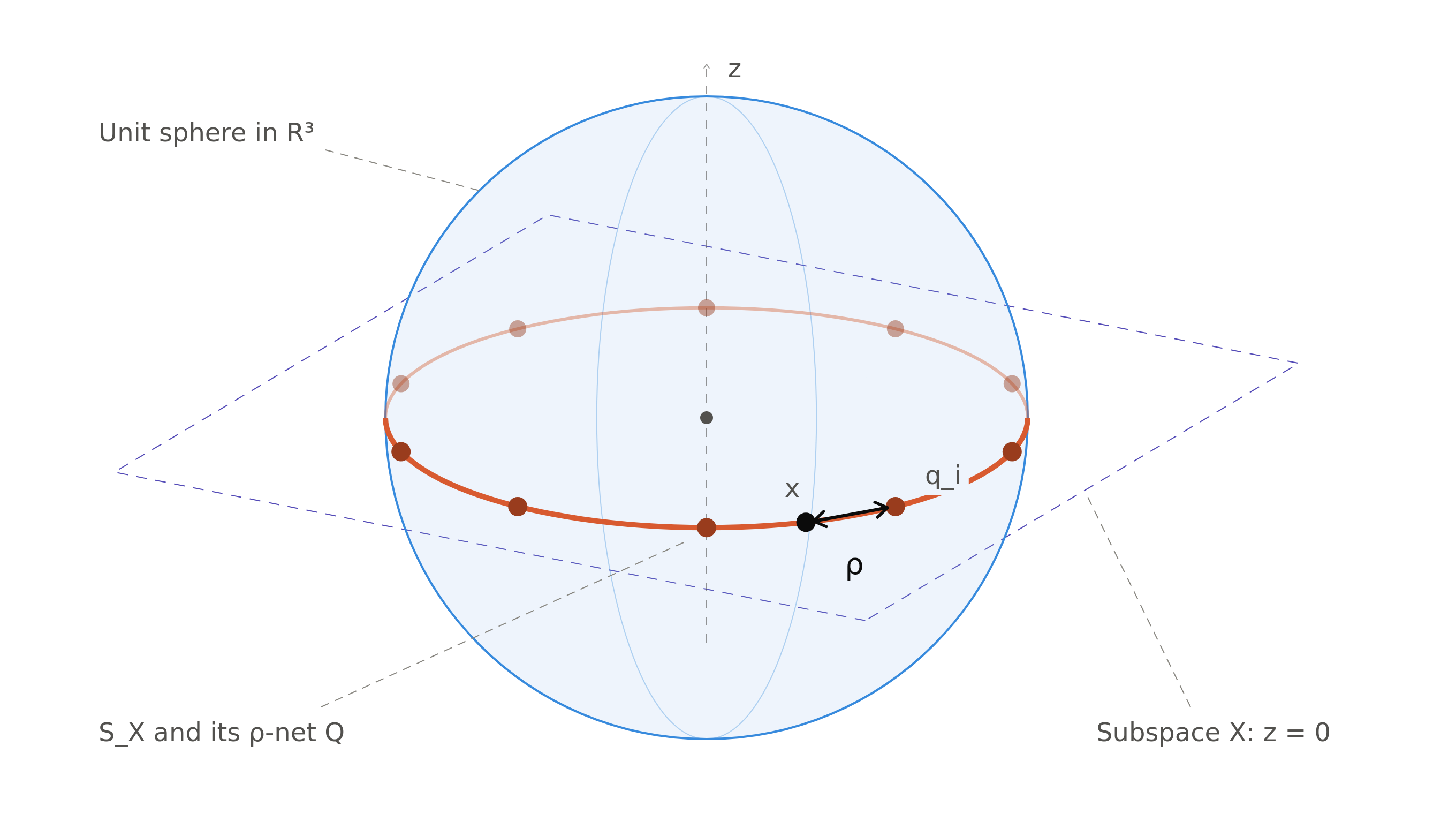
Let $X \subseteq \mathbb{R}^N$ be a $k$-dimensional linear subspace, and let $S_X = \{ x \in X ~ | ~ \lVert x \rVert_2 = 1 \}$ be its unit sphere. A finite set $Q \subseteq S_X$ is a $\rho$-net of $S_X$ if $$ \min_{q \in Q} \lVert q - x \rVert_2 \leq \rho \quad \text{for all } x \in S_X . $$ Furthermore, For every $\rho \in (0,1)$ there exists a $\rho$-net with cardinality $|Q| \leq (3/\rho)^k$.
To justify this cardinality, firstly note that that the volume of any ball $B(c,r) = \{ y \in X : \lVert y - c \rVert_2 \leq r \}$ equals $\kappa_k r^k$ for some $\kappa_k$ that depends only on $k$. Secondly, note that if we keep packing balls of radius $\tfrac{\rho}{2}$ at an exact distance of $\tfrac{\rho}{2}$, until we cannot pack any more, they will a) fit inside the larger $B(0, 1 + \tfrac{\rho}{2})$ ball, b) be non-overlapping, and c) every $x \in S_X$ will be at most at $\rho$ distance. Thus we have:
$$ \begin{align*} & |Q| \kappa_k \Big(\frac{\rho}{2} \Big)^k = |Q| ~ \text{Vol}\big[B \Big(q, \frac{\rho}{2} \Big) \Big] \stackrel{!}{\leq} \text{Vol}\Big[B \Big(0, 1 + \frac{\rho}{2} \Big) \Big] = \kappa_k \Big( 1 + \frac{\rho}{2} \Big)^k \\ & \Rightarrow |Q| \leq \frac{\kappa_k \Big( 1 + \frac{\rho}{2} \Big)^k}{\kappa_k \Big(\frac{\rho}{2} \Big)^k} = \Big( \frac{2 + \rho}{\rho} \Big)^k \leq \Big( \frac{3}{\rho} \Big)^k \end{align*} $$
With this, we have all elements needed to derive the main results from [BDDW08]: probabilistic bounds for the RIP of subgaussian matrices for fixed and arbitrary $k$-sparse $x$, and subsequent measurement bounds.
Let $\Phi \in \mathbb{R}^{n \times N}$ be a random matrix with independent centered entries with variance $\mathbb{E}[\phi_{ij}^2] = 1/n$ and subgaussian tail bounds (with scale parameter $K$). Then, for all $k$-sparse $x$ simultaneously, and for $\delta \in (0, 1)$, the RIP: $$ (1 - \delta) \lVert x \rVert_2 \leq \lVert \Phi x \rVert_2 \leq (1 + \delta) \lVert x \rVert_2 $$ Holds for constants $c_1=12e$ and $c_2 > 0$ depending only on $K$, with probability of at least $$ 1 - 2 \exp\Big(k \log \Big( c_1 \frac{N}{k \delta} \Big) - c_2 n \delta^2 \Big) $$
And thus, for a fixed $\delta$ and $n = \mu k \log (\frac{c_1}{\delta} \frac{N}{k} )$ with $\mu > 1 / (c_2 \delta^2)$, the exponent becomes: $$ -\eta := -\big( c_2 \delta^2 \mu - 1 \big) k \log \Big( \frac{c_1}{\delta} \frac{N}{k} \Big) $$ and thus for $n \asymp k \log(N/k)$, $\Phi$ satisfies the RIP with probability of at least $1 - 2 e^{-\eta}$.
To see this, consider the set of all unit norm vectors with a particular (fixed) $k$-sparse support. By our definitions before, this is an instance of $S_X$, the unit sphere of a $k$-dimensional linear space. We will also make use of $Q$, the $\rho$-net of $S_X$, composed by at most $(3 / \rho)^k$ unit norm vectors (recall: $\rho \in (0, 1)$).
We start observing that, for each fixed $q \in Q$ (and for $0 < \epsilon < 1$), the matrix $\Phi$ satisfies the following inequality (using $\lVert q \rVert_2 = 1$ and the probability tail bound from before): $$ \begin{align*} P\big( \lVert \Phi q \rVert_2 \notin & [1-\epsilon, 1+\epsilon] \big) \leq P\big( \lVert \Phi q \rVert_2^2 \notin [1-\epsilon, 1+\epsilon] \big) \\ = &P\big( \big| \lVert \Phi q \rVert_2^2 - \lVert q \rVert_2^2 \big| \geq \epsilon \lVert q \rVert_2^2 \big) \leq 2 \exp\Big( -cn \frac{\epsilon^2}{\nu^2 \kappa^4} \Big) \end{align*} $$ Since we know the cardinality of $Q$, we can bound the probability of isometry for the best element over all $Q$, via union bound and complement: $$ P(\lVert \Phi q \rVert_2 \in [1 - \epsilon, 1 + \epsilon]) \geq 1 - 2 \Big( \frac{3}{\rho} \Big)^k \exp \Big( -cn \Big(\frac{\epsilon^2}{ \nu^2 \kappa^4} \Big) \Big) $$
Another quite useful property of $Q$ is that, for reasonable values of $\epsilon, \rho$, the above is “already enough” to extend the above bound from $Q$ to all of $S_X$. To show this, first define $A$ as the smallest number such that $\lVert \Phi x \rVert_2 \leq (1 + A) \lVert x \rVert_2 = 1 + A$ for all $x \in S_X$ (this also applies to $\lVert \Phi (x - q) \rVert_2 \leq (1 + A) \rho$, since $q$ is also in $S_X$). By the triangle inequality and definition of $Q$, the following bound for $A$ holds with the above probability: $$ \begin{align*} &\lVert \Phi x \rVert_2 \leq (1 + A) \leq \underbrace{\lVert \Phi q \rVert_2}_{\leq 1 + \epsilon} + \underbrace{\lVert \Phi (x - q) \rVert_2}_{\leq (1 + A)\rho} \leq 1 + \epsilon + (1 + A)\rho \\ \Rightarrow & (1 + A) (1 - \rho) \leq 1 + \epsilon \Rightarrow A \leq \frac{1 + \epsilon}{1 - \rho} - 1 \Rightarrow A \leq \frac{\epsilon + \rho}{1 - \rho} \end{align*} $$ Now, let’s say we want to satisfy the RIP for some $\delta \in (0, 1)$. If we choose the density of our net to satisfy $\rho = \frac{\delta}{4}$, and set our tail bound threshold to $\epsilon = \frac{\delta}{2}$, we get the desired $A \leq \delta$ bound (also applying $1 - \delta/4 \geq 3/4$): $$ A \leq \frac{\delta/2 + \delta/4}{1 - \delta/4} \leq \frac{3 \delta/4}{3/4} = \delta $$ From this, we can also obtain the lower bound: $$ \begin{align*} \lVert \Phi x \rVert_2 \geq \underbrace{\lVert \Phi q \rVert_2}_{\geq 1 - \delta/2} - \underbrace{\lVert \Phi (x - q) \rVert_2}_{\geq (1 - \delta)\frac{\delta}{4}} \geq 1 - \frac{\delta}{2} - \frac{\delta}{4} + \frac{\delta^2}{4} \geq 1 - \delta \end{align*} $$ And thus we obtain probability bounds that apply for every $x \in S_X$ (replacing $\epsilon$ and $\rho$): $$ \begin{align*} P(\lVert \Phi x \rVert_2 \in [1 - \delta, 1 + \delta]) \geq &1 - 2 \Big(\frac{12}{\delta} \Big)^k \exp \Big( -cn \Big(\frac{\delta^2}{2^2 \nu^2 \kappa^4} \Big) \Big)\\ &\text{For every $x \in S_X$.} \end{align*} $$
But this result only applies to $k$-sparse vectors on one particular, fixed support. There are $\binom{N}{k} \leq (eN / k)^k$ distinct subspaces like $S_X$ inside of $\mathbb{R}^N$. To obtain isometry guarantees for all $k$-sparse vectors jointly, we can apply one last union bound:
$$ \begin{align*} P(\lVert \Phi x \rVert_2 \in [1 - \delta, 1 + \delta]) \geq &1 - 2 \Big(\frac{eN}{k}\Big)^k \Big(\frac{12}{\delta} \Big)^k \exp \Big( -cn \Big(\frac{\delta^2}{2^2 \nu^2 \kappa^4} \Big) \Big)\\ &\text{For every $k$-sparse $x$.} \end{align*} $$
We can also obtain the associated measurement bounds. Regrouping parameters we get: $$ \begin{align*} &\Big(\frac{eN}{k}\Big)^k \Big(\frac{12}{\delta} \Big)^k \exp \Big( -cn \Big(\frac{\delta^2}{2^2 \nu^2 \kappa^4} \Big) \Big) \\ = &\exp \Big(k \log \Big( \underbrace{12e}_{c_1} \frac{N}{k \delta} \big) - \Big(\underbrace{\frac{c}{4 \nu^2 \kappa^4}}_{c_2} n \delta^2 \Big) \Big) \end{align*} $$ For the bound to be useful, the exponent needs to be negative: $$ k \log \Big( c_1 \frac{N}{k \delta} \Big) \leq c_2 n \delta^2 \Rightarrow n \geq \frac{1}{c_2 \delta^2} k \log \Big( c_1 \frac{N}{k \delta} \Big) $$ Yielding the final measurement bounds.
A small detail missing: we proved this for all $k$-sparse $x$ with unit norm, but it is easy to show the statement applies to $k$-sparse $x$ of all norms. Let $x’ = \xi x$ for any $\xi > 0$. Then, $\lVert x’ \rVert_2 = \xi$ and $$ \lVert \Phi x \rVert_2 \in [1 - \delta, 1 + \delta] \iff \frac{\lVert \Phi \xi x \rVert_2}{\xi} \in [1 - \delta, 1 + \delta] \iff \lVert \Phi x’ \rVert_2 \in [(1 - \delta) \lVert x’ \rVert_2, (1 + \delta) \lVert x’ \rVert_2] $$
The green box is a bit of a mix-match of results. To summarize,
- We sample $\Phi$ from a broad family of iid subgaussian random matrices
- We show that $\Phi$ is isometric on a discrete, fixed-support set $Q$
- This isometry extends naturally to the continuous, fixed-support set $S_X$
- Through union bounds and rescaling, this extends to an isometry bound on all $k$-sparse inputs
- Forcing this bound to have a negative exponent yields the desired measurement bounds
-
The [BDDW08] paper also includes a nice discussion showing that the $\mathcal{O}(k \log(N/k))$ measurement bound is optimal, since it is bounded by the Gelfand width of $\ell_p$ balls. In that sense, this derivation is optimal. Still, further useful results and sharper constants can be found in Chapter 9 from the CoSe book also provides sharp and useful results in a clear manner.
-
This often-called “covering-net” technique can also be applied to other settings with great success. For instance, here used it to prove that a random linear operator $\mathcal{A}: \mathbb{R}^{a_1 \times a_2} \to \mathbb{R}^b$ also satisfies the rank-RIP and permits the efficient recovery of rank-$k$ matrices from few measurements. In this case, it is interesting that the measurement bound is $\mathcal{O}((a_1 + a_2) k)$, and not $\mathcal{O}((a_1 + a_2) k \log((a_1 + a_2) / k))$. No log-factor is needed! This is because the $\log(N/k)$ factor in the vector case comes from the (combinatorial) union bound over $k$-sparse supports, whereas rank-$k$ matrices can be fully characterized by a single manifold (Grassmannian) that admits a $\rho$-net of cardinality $\mathcal{O}(\exp((a_1 + a_2)k \log(1 / \rho)))$.
Recapping Ideas
$P_0$ reduces to an intractable problem, but we rest in peace reassured that the isometry of $P_1$ reliably identifies the precise result: intensities paired with their respective indices. Particularly, random independent projections reach inordinate probabilities of rendering isometries (provided randomness is properly realized), increasing practicality and resulting in a procedure of relevance and interest for plenty of research and industry projects.