Compressed Sensing
Motivation
When sharing my passion about Compressed Sensing (CoSe) (Candès, Romberg, Tao, 2004), I found that it is sometimes a difficult topic to introduce, even to qualified people, mainly for the following reasons:
- Its results are very general and powerful, but this isn’t always obvious or intuitive
- Applications are not abundant in our daily life or easy to explain (e.g. involving Fourier scattering in magnetic resonances)
- The elements and techniques involved are relatively diverse (e.g. Restricted Isometry Property and $\ell_1$ relaxations)
Due to the first point, even when the CoSe principles are understood, they can be sometimes hard to believe. I decided to write this post to help myself and others understanding, believing and loving CoSe, by:
- Providing support materials (references, figures, explanations) and intuitions to get a grip on CoSe
- Providing computational experiments to show that it actually works
- Discussing some powerful implications
Still, it is worth mentioning that, since it crystalized in 2004, a wealth of divulgational resources on the topic have been written, by much more qualified people than me, and with more rigorous and comprehensive coverage, for example:
- Candès and Wakin (divulgational paper): https://ieeexplore.ieee.org/document/4472240
- Terry Tao (divulgational blog): https://terrytao.wordpress.com/tag/compressed-sensing/
- Igor Carron: https://nuit-blanche.blogspot.com/
Absolutely recommended reads! There was also a lot of literature on sparse recovery prior to 2004 that led to those results. More references are also briefly presented throughout this post and at the end.
From compression to compressed sensing
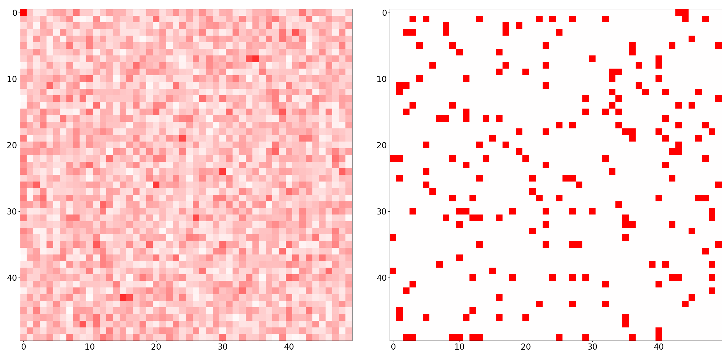
One natural starting point is comparing CoSe with regular compression. Let’s consider a discrete signal represented by the vector $s(x) \in \mathbb{C}^{D}$ where $s(x) \neq \vec{0}~$ for $T \ll D$ values of $x$, and $0$ for the rest (i.e. $s$ is $T$-sparse), like the matrix depicted here on the left:
Now, given $s$, we can compress it (i.e. store it in a way that takes less than $50\times50=2500$ entries) without any loss of information, e.g. by storing the $(x_1, x_2)$ location and value of each non-zero entry, resulting in a compressed version $\overline{s}$ with a total of 30 entries. To reconstruct $s$ from $\overline{s}$, we would just need to create a “blank” $50\times50$ matrix, and fill each of the entries matching its location and value. It is easy to see that the size of the compressed representation depends only on $T$, which is potentially much smaller than $D$.
But note that we still needed to know all $D$ entries to obtain $\overline{s}$. This can be extremely disadvantageous when the inspection or storage of $D$ is infeasible (e.g. due to time, memory or physical constraints). This is our first major takeaway from CoSe:
In this sense, we can regard it as the inverse problem of compression, specifically in the family of linear coding.
Much more powerful than it looks
At first sight, CoSe may look like a convenient way of saving memory and/or sensing resources. But it has much deeper implications:
Imagine that there is a 1-megapixel picture of the night sky, pitch black everywhere except for $T=10$ stars that appear at random pixels with random intensities. The claim is that we are almost certain to perfectly resconstruct each of the 1 million pixels, including the exact position and brightness of the stars, by doing in the order of $M \approx 100$ measurements.
This looks like a combinatorial problem, doesn’t it? Even disregarding the intensities, we have $\binom{10^6}{10}$ combinations, and only $\sim 100$ datapoints. But even better: the number of measurements needed wouldn’t change even if we had 1 billion pixels, or more generally $\binom{D}{T}$ combinations for any arbitrarily large $D$. How can we know the locations and intensities if all we ever had is $M$ measurements? Also, shouldn’t the reconstruction quality depend on the image size $D$?
Let’s say I store a marble in one of 2 cups. To encode the location, I need 1 bit. Now, if I store the marble in one of 8 cups, I need 3 bits instead.
So even if my sparsity is $T=1$ in both cases, the amount of information in this sparse signal increases with $log(D)$. Wouldn’t a recovery method with measurements that don’t depend on $D$ violate some law of information conservation, allowing us to “create more information” just by artificially increasing $D$ (i.e. “adding more empty cups”)?
Indeed, it seems that such a perfect recovery sounds too good to be true and/or would go against our intuitions. But the key to make this work lies in the following 2 conditions:
- We assume/know that the signal we want to recover is sparse
- The $M \approx T log(T)$ measurements we make are sufficiently incoherent against the sparse signal’s distribution
Let’s start discussing the first condition. Just keep in mind that the second condition (discussed afterwards) is assumed to be fulfilled.
1. Sparse solutions
Since we have a $D$-dimensional signal, but we only took $M \ll D$ measurements (for $M$ in the order of $T log(T)$), it is intuitive to see that we have $D-M$ degrees of freedom (a so-called underdetermined system), leading generally to infinitely many solutions $\hat{s}$ that would fit our measurements.
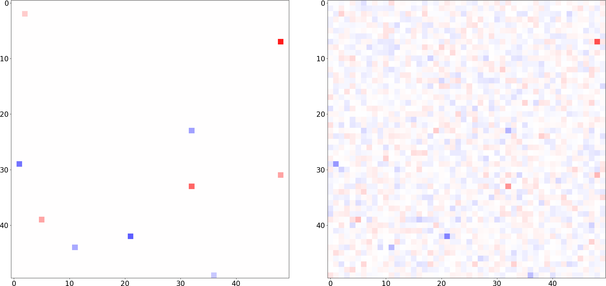
In the figure below we show one of them: Given our sparse matrix $s$ from before, we took $M=200$ random Fourier measurements, set the rest to zero, and computed the inverse FT. The result is a naïve solution $\hat{s}$ that kind of resembles the original, and is perfectly consistent with our partial measurements, but one thing pops to the eye: the recovery is not correct, and it is not sparse: 😤
But how to find those sparse solutions? Luckily for us, we know that “for most large underdetermined systems of linear equations the minimal $\ell_1$-norm solution is also the sparsest solution” (Donoho, 2006). So we slightly modify our task: the plan is to find the $\hat{s}$ with minimal $\ell_1$ norm that is consistent with our measurements $m \in \mathbb{C}^M$, since this will likely yield the sparsest consistent $\hat{s}$:
$$ \hat{s}_1 \quad = \quad \operatorname*{argmin}_x \quad \lVert x \rVert_1 \quad s.t. \quad \Phi^* x = m $$
Where $\Phi \in \mathbb{C}^{D \times M}$ is our so-called sensing matrix (that leads to the measurements we take), assumed to be sufficiently incoherent (discussed later).
This is one of the prime contributions from CoSe: Given an adequate sensing matrix $\Phi$, the seminal CoSe papers prove that this $\ell_1$-sparsest solution has an almost certain probability of the following:
- Existing
- Being unique
- Being our desired solution
All great news across the board! The literature also deals with characterizing and finding good values of $\Phi$. Furthermore, the solution is also robust to noise, so the noiseless toy-examples from this post extend to real-world scenarios.
Computationally, $\ell_1$ is a fantastic way of enforcing our sparsity prior, because finding $\hat{s}_1$ efficiently amounts to solving a Linear Program. Very good LP solvers are widely implemented, and the code is relatively simple. I wrote a Python script (full script here, and also online) that demonstrates the perfect recovery of a randomly sparse signal for widely varying $D$, but fixed $T$ and $M$. It is released under MIT license, so feel free to play around with it! The snippet below illustrates the main routine:
# define globals, you can play around with these parameters
dim1, x1, y1 = 51,        3,  372.32839
dim2, x2, y2 = 10_000, 8173, -537.72937
measurement_idxs_1 = (2, 7, 8, 10,
                      11, 18, 19, 20)
measurement_idxs_2 = (69, 1233, 1782, 2022,
                      4205, 6794, 9902, 9997)

# create two signals of different lengths but with same sparsity level
original1 = np.zeros(dim1)
original1[x1] = y1
original2 = np.zeros(dim2)
original2[x2] = y2

# gather random FFT CoSe matrices for s1 and s2.
# These matrices are "tall":
# the height corresponds to the length of the original signals, which
# varies, but the width to the (much smaller) number of measurements
cosemat1 = get_dft_coefficients(dim1, *measurement_idxs_1)
cosemat2 = get_dft_coefficients(dim2, *measurement_idxs_2)

# perform "measurements", which is equivalent to computing dotprods
# between original signal and each basis from the cose matrices.
# note that both measurements have same length, despite the length
# differences between original1 and original2
measurements1 = cosemat1.T @ original1
measurements2 = cosemat2.T @ original2

# this is the interesting step. Given the (short) measurements,
# our sensing matrices and the original length of the signal (all
# things we readily know), we recover the original signal exactly!
# i.e. all zeros except ori[x] = y, with the exact location and value
# of the spike. This is true regardless of the length of the original!
recovery1 = cose_recovery(dim1, measurements1, cosemat1)
recovery2 = cose_recovery(dim2, measurements2, cosemat2)

# Finally, check that recovered signals are equal to originals
assert np.allclose(original1, recovery1), "This should not happen!"
assert np.allclose(original2, recovery2), "This should not happen!"
print("Recovered signals were identical!")
To finalize bringing the point home, the figure below illustrates the impact of $\ell_1$ towards sparsity:
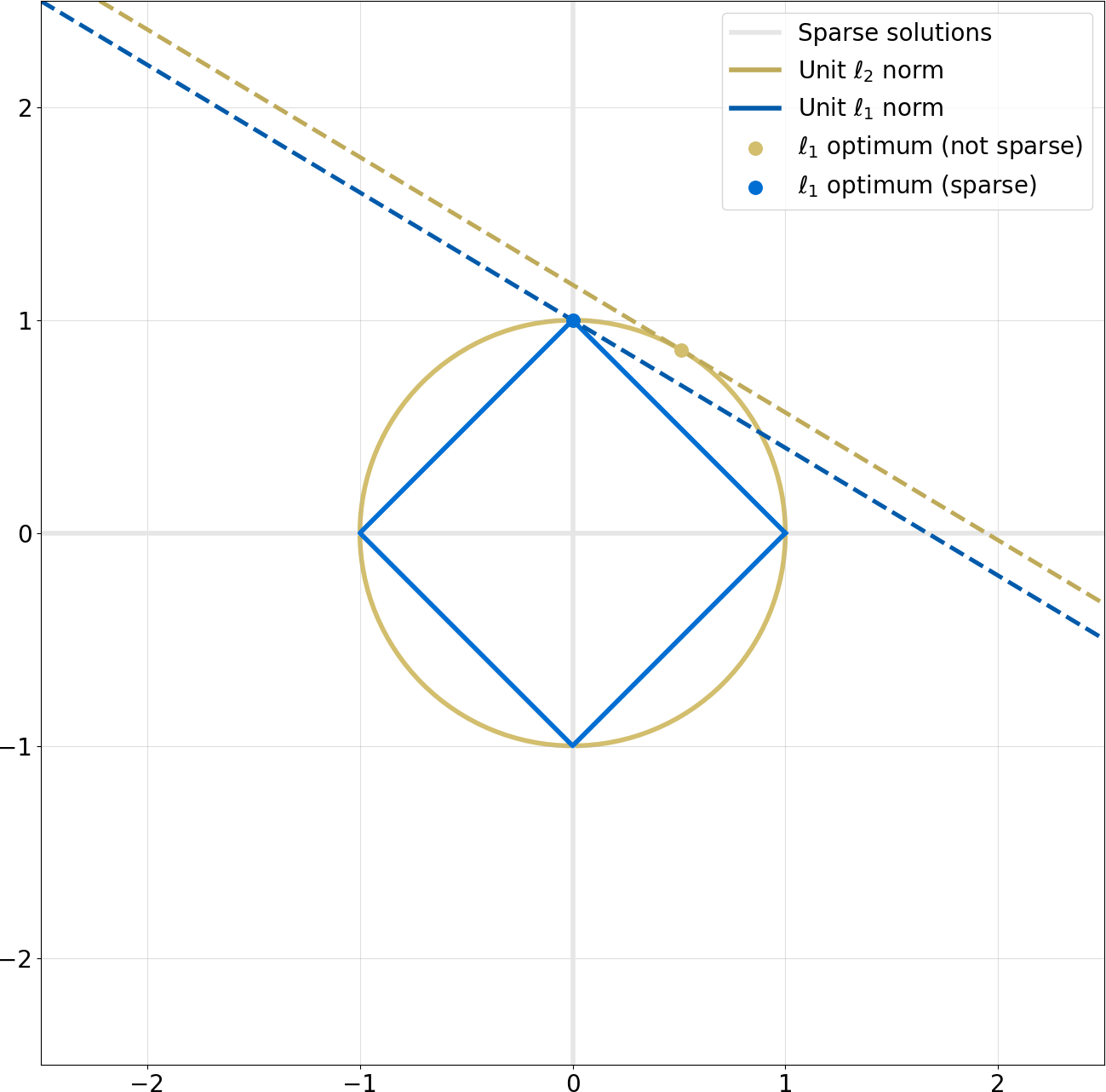
The interpretation is as follows:
- The circle and diamond illustrate all solutions in $\mathbb{R}^2$ with the same norm in $\ell_2$ and $\ell_1$, respectively. We can imagine this norm is our $\operatorname*{min}~\lVert x \rVert_1$ (here we set it to 1, but could be any other positive value depending on our specific $\Phi, m$)
- The lines belong to a subspace of $\mathbb{R}^2$ that matches some constraint (e.g. a specific slope). This is underdetermined: we have infinitely many lines in $\mathbb{R}^2$ with that slope.
- The dots correspond to “minimal norm” solutions ($\ell_2$ and $\ell_1$ respectively) that satisfy the slope constraint: all other points in the lines have higher norms.
- We observe that the $\ell_1$ solution lies on the vertical origin, i.e. it is sparse (because the horizontal value is zero), while the $\ell_2$ one isn’t. Furthermore, almost every slope leads to a sparse $\ell_1$ solution, while almost every slope leads to a non-sparse $\ell_2$ solution.
This last point is the reason why we have an “almost certain” chance of recovering the sparsest solution if we do a random (and incoherent) measurement, represented here by picking a random slope.
Remember that our system is underdetermined because we have less measurements $M$ than signal dimensions $D$. This is represented here by the fact that the points in the diamond/circle correspond to 2-dimensional signals, whereas the 1-dimensional line corresponds to the constraints from a single measurement $\Phi^* x = ax_1 + bx_2 = m \in \mathbb{C}$.
More generally, we can imagine that the diamond lives in a $D$-dimensional space as a cross-polytope, representing the space of possible $\hat{s}$ solutions, and the lines live in the lower $M$-dimensional space as hyperplanes, representing our underdetermined measurements $\Phi^* s = m$. The point where a hyperplane touches the minimal-norm polytope is our optimal solution $\hat{s}_1$.
Now we can intuitively see that, even if we maintain the dimensionality of the hyperplane $M$, increasing the dimensionality $D$ of the cross-polytope would still expose a “corner”, and we are still almost certain to find it by solving our LP.
2. Incoherent measurements
Throughout the last section, we’ve assumed that our measurements are sufficiently incoherent, as a condition for the validity of the conclusions. But what do we mean with sufficiently incoherent?
We’ll first try to get some intuition, and then review the more rigorous definition.
Intuition
Let’s revisit our previous example in which we take a 1-megapixel picture $s$ of a sky that is pitch black, except for $T=10$ stars that appear at random pixels with random intensities. We claimed that $M \approx 100$ measurements would help us recover the support of $s$ out of $\binom{10^6}{10}$ combinations, even with correct intensities, and we’ve provided intuitions and Python code showing that this actually works.
Now, when we think about a single measurement, our first intuition is to think of a single pixel. But this would be bad. Observe the image below:
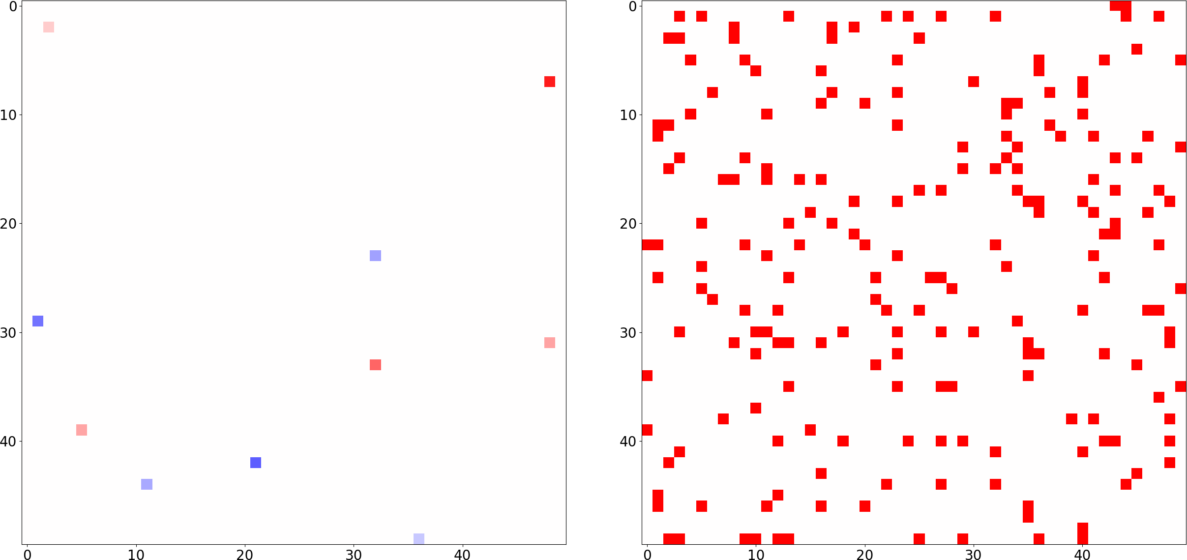
Here, each measurement is equivalent to a question: “what is the value of the signal for this pixel?” And the most likely answer for each question will be “it is zero”. So we would get many zero-measurements, and with that information, low hopes of correctly recovering $s$.
In the extreme case, there would be no overlap and we would get all zero measurements, i.e. $\Phi^* x = 0$. This would lead to the LP solution $\hat{s} = 0$, which is clearly incorrect since we know our signal has non-zero entries.
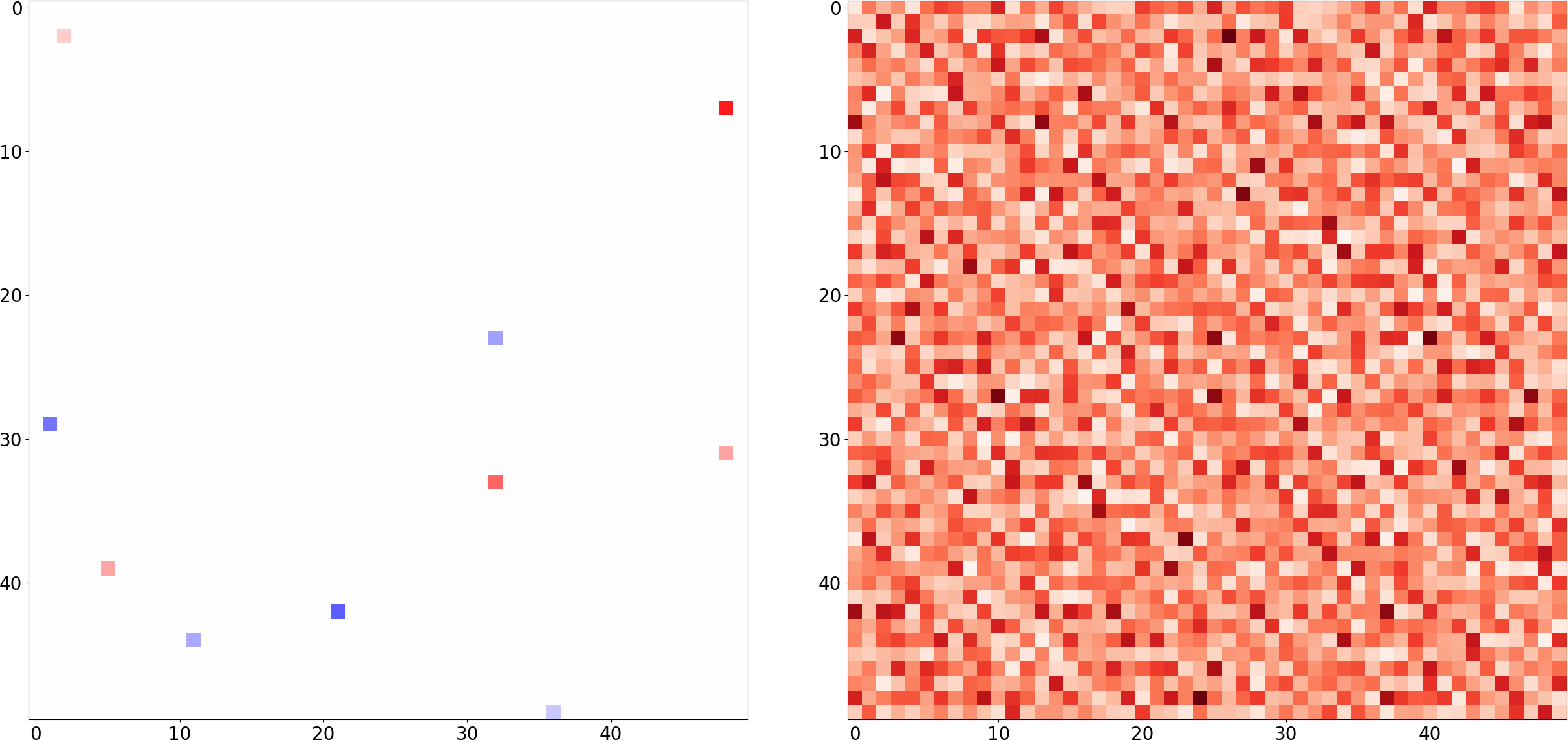
Now let’s look at a “different measurement space”. In our examples, we used random Fourier measurements, illustrated in the image below:
Here, we make the same number of measurements (right image), but on the Fourier basis. I.e. instead of asking “what is the value of the signal for this pixel?”, we ask “what is the value of the signal for this frequency component?”. And we do this for 200 random frequency components.
The left image shows the distribution of our measurement basis when we project it on the pixel space. Since each frequency component oscillates periodically, the sum of the 200 random components covers the full image in a dense and noisy manner.
Intuitively, you can think of this as a kind of “holographic” information: each measurement tells us a bit about every pixel, but not much about any specific pixel (Fourier basis). On the other hand, pixel measurements tell us everything about a single pixel but nothing about the others (Dirac basis).
In a way, these 2 bases are completely “opposed”: this is what we mean by sufficiently incoherent. Paradoxically, this is exactly what we want, since all measurements are likely to be informative, by interacting with the non-zero elements of $s$, and the $\ell_1$ optimal solution is almost certain to exist, be unique and correct (proofs given in the papers).
Note that this would also work the other way around (i.e. if a signal is sparse in the frequency space, we would be OK doing random pixel-wise measurements), or with other families of bases.
More generally, the intuition is that if our signal $s$ is sparse on a given basis $\mathcal{B}$, then our measurement matrix $\Phi$ should come from a basis that is sufficiently “different” from $\mathcal{B}$. In CoSe, this is characterized by the Restricted Isometry Property (RIP), introduced in (Candès, Tao, 2005), and revisited and developed in (Candès, 2008).
The RIP 💀
Formally, we say that our measurement matrix $\Phi$ satisfies the RIP with $\delta \in [0, 1]$ if the following holds for all $x \in \mathbb{C}^D$ (including all possible levels of sparsity $T \in \{ 1, \dots, D \} $), and for all possible $\Phi_{sub}$ column combinations of $\Phi$:
$$
(1 - \delta)\lVert x \rVert_2^2~~\leq~~\lVert \Phi_{sub}^* x \rVert_2^2~~ \leq ~~(1 + \delta)\lVert x \rVert_2^2\\
$$
Furthermore, the isometry constant $\delta_{iso}$ is defined as the smallest $\delta$ for which the RIP holds.
As defined here, the RIP is a bound on how much does $\Phi$ modify the length of any given $x$ (Note the similarity in formulation to the Johnson-Lindenstrauss Lemma).
One equivalent interpretation of the RIP is that all eigenvalues of $\Phi^* \Phi$ are in the interval $[(1 - \delta), (1 + \delta)]$. With this interpretation, a $\Phi$ with orthonormal columns would lead to the smallest possible $\delta_{iso}$. As it can be seen in (Candès, 2008), a small $\delta_{iso}$ is desirable. Intuitively, this makes sense, because the less we alter the norm of $x$, the less chances of an alias we have, hence our LP solution has more chances of being unique (and sparse+correct).
Note that the RIP inequalities must hold for all possible $\Phi_{sub}$. Let’s assume we have a $T=1, D=4$ sparse signal $s$ on the Dirac (standard) basis $\mathcal{D}$, e.g.:
$$ x = \begin{pmatrix} 0\\ 1\\ 0\\ 0\\ \end{pmatrix} $$
Now, let’s take a look at the Dirac (standard) basis $\mathcal{D}$ against the Fourier basis $\mathcal{F}$:
$$ \mathcal{D} := \begin{pmatrix} \color{fuchsia}{1} & 0 & \color{fuchsia}{0} & \color{fuchsia}{0}\\ \color{fuchsia}{0} & 1 & \color{fuchsia}{0} & \color{fuchsia}{0}\\ \color{fuchsia}{0} & 0 & \color{fuchsia}{1} & \color{fuchsia}{0}\\ \color{fuchsia}{0} & 0 & \color{fuchsia}{0} & \color{fuchsia}{1}\\ \end{pmatrix} \quad \mathcal{F} := \frac{1}{2}\begin{pmatrix} \color{fuchsia}{1} & 1 & \color{fuchsia}{1} & \color{fuchsia}{1}\\ \color{fuchsia}{1} & -i & \color{fuchsia}{-1} & \color{fuchsia}{i}\\ \color{fuchsia}{1} & -1 & \color{fuchsia}{1} & \color{fuchsia}{-1}\\ \color{fuchsia}{1} & +i & \color{fuchsia}{-1} & \color{fuchsia}{-i}\\ \end{pmatrix} $$
It is true that both matrices are orthogonal, but what happens with their RIP if we now pick the first, third and last columns (highlighted)?
$$
\mathcal{D}_{sub}^* x = \begin{pmatrix}
\color{fuchsia}{1} & \color{fuchsia}{0} & \color{fuchsia}{0} & \color{fuchsia}{0}\\
\color{fuchsia}{0} & \color{fuchsia}{0} & \color{fuchsia}{1} & \color{fuchsia}{0}\\
\color{fuchsia}{0} & \color{fuchsia}{0} & \color{fuchsia}{0} & \color{fuchsia}{1}\\
\end{pmatrix}
\begin{pmatrix}
0\\ 1\\ 0\\ 0\\
\end{pmatrix} =
\begin{pmatrix}
0\\ 0\\ 0\\
\end{pmatrix}
$$
We see that the $\delta$ for this case must be 1, since $(1 - \delta) \lVert x \rVert_2^2 \leq \lVert \mathcal{D}_{sub}^* x \rVert_2^2 = 0$.
This is exactly the case that we mentioned before, where our pixel-mask would not overlap with $s$, leading to the ill-posed $\Phi^* x = 0$ constraint!
Crucially, this is not the case for $\mathcal{F}$: here, $\delta$ will be minimal for any possible combination of columns, and so will $\delta_{iso}$. So, ideally, our sensing matrix $\Phi$ would be:
- Closest to orthogonal
- Have a distribution of columns that doesn’t correlate well with the basis on which $x$ is sparse.
This, in essence, is the meaning of incoherence, and the RIP is the CoSe way of quantifying it.
The bottom line for this section is that, all the nice results and implications are true, as long as we are able to put a finger on the sparse basis $\mathcal{B}$, and to find an appropriate measurement matrix $\Phi$ (i.e. incoherent). This means that CoSe can solve many problems of combinatorial nature, but not nearly all: incoherence must be satisfied.
Actually, if we go back and take a look at our naïve reconstruction, we see that it is already fairly close to the actual solution, so it is not that we are solving a wildly combinatorial, cryptographic task: a lot of the “heavy lifting” is done by having a proper choice of $\Phi$, and $\ell_1$ “brings it home”. In fact, the proof in the original CoSe paper relies on this “fairly close” property, by constructing a polynomial that respects certain bounds on the support of $s$ (see sections 2.2 and 3).
So it is understandable that a lot of the CoSe literature is about characterizing and finding good $\Phi$. There are families of random matrices with advantageous properties, but unfortunately, it turns out that figuring out the cases for which $\Phi$ has a satisfactory RIP is $NP$-hard (Bandeira et al., 2012). So while the CoSe framework is tremendously powerful, it has limitations and particularly it can’t be used to solve arbitrary combinatorial tasks or to tackle the $P \neq NP$ problem.
Final thoughts and further sources
Hopefully, we succeeded in providing satisfactory intuition and examples involving CoSe, and as a consequence, we now know and understand the main elements involved, how/when they lead to exact recovery, and the scope and extent of the main results. Here is a final breakdown:
- We assume that the signal $s \in \mathbb{C}^D$ is $T$-sparse on a given basis $\mathcal{B}$
- We take $M = \mathcal{O}(T log(T)), M \ll D$ measurements on a basis $\Phi$ that is incoherent to $\mathcal{B}$, and we want to recover $s$.
- Among the many solutions $\hat{s}$ consistent with our measurements, we pick $\hat{s}_1$ with minimal $\ell_1$ norm satisfying $\Phi^* \hat{s}_1 = m$.
- If $\Phi$ satisfies the RIP, $\hat{s}_1$ exists, is unique, and is identical to $s$ with an almost certain probability
- This allows us to effectively recover sparse signals embedded in very high-dimensional spaces, saving resources, and overcoming combinatorial search spaces, with almost certain probability.
There is of course much more worth discussing, for example:
- Applications as well as possible relations to Deep Learning (Unser, 2020), (Bora et al., 2017), (Mundt et al., 2021), (Papyan, Romano, Elad, 2017), (Voulgaris, Davies, Yaghoobi, 2020), (Zhang, Titov, Sennrich, 2021)
- Extensions to noisy scenarios (Candès, Romberg, Tao, 2005)
- Usage and characterization of structured random matrices for $\Phi$ (e.g. Rauhut, 2011)
- Extensions to further measurement bases, like noiselets; discussion on known sparsity-exposing bases like wavelets (Daubechies, 1988), (Mallat, 1989) and Robust PCA (Candès et al., 2009)
- Alternative strategies to $\ell_1$, e.g. greedy methods like OMP (Pati, Rezaiifar, Krishnaprasad, 1993) or CoSaMP (Needell, Tropp, 2008)
- Discussion of Tao’s refined uncertainty principle and the optimality of the $M = \mathcal{O}(T log(T))$ bound
- Model-based CoSe yielding $M = \mathcal{O}(T)$ for certain families of signals (e.g. wavelets) (Baraniuk et al., 2008)
- CoSe characterization of different algorithms from the literature (e.g. (Satpathi, Das, Chakraborty, 2013), (Mukhopadhyay, Satpathi, Chakraborty, 2015))
- Revision of relevant literature prior to CoSe, e.g.:
- Discussion on $\ell_1$ relaxations: Basis Pursuit (Chen, Donoho, Saunders, 1998)
- $NP$-Hardness and intractable combinatorial nature of $\ell_0$, the sparse recovery problem ((Natarajan, 1995), extended to non-negative by (Nguyen et al., 2019))
- RIP precursors: Mutual incoherence (Donoho, Huo, 2001), Babel function (Tropp, 2004)
Hopefully I’ll have the chance to elaborate on some of them in future posts (let me know if you find any particularly interesting!). For the moment, this list is sparse in details to keep the size of this post sensibly compressed 💾, otherwise this post will have a…
Ok, now no more puns! Thanks for…